
Intel® Cluster Toolkit Compiler Edition 4.0 for Linux* OS
Getting Started Guide
Copyright © 2003–2010 Intel Corporation
All Rights Reserved
Document Number: 318537-006
Revision: 20100602
World Wide Web: http://www.intel.com
Disclaimer and Legal Information
2................... Introduction
3................... Intel Software Downloads, Installation, and Uninstalling on Linux* OS
4................... Getting Started with Intel® MPI Library
4.2 How to Set Up MPD Daemons on Linux* OS
4.3 The mpdboot Command for Linux* OS
4.4 Compiling and Linking with Intel® MPI Library on Linux* OS
4.5 Selecting a Network Fabric
4.6 Running an MPI Program Using Intel® MPI Library on Linux* OS
4.7 Experimenting with Intel® MPI Library on Linux* OS.
4.8 Controlling MPI Process Placement on Linux* OS
4.9 Using the Automatic Tuning Utility Called mpitune
4.9.2 MPI Application-Specific Tuning
4.10 Extended File I/O System Support on Linux* OS
4.10.1 How to Use the Environment Variables I_MPI_EXTRA_FILESYSTEM and I_MPI_EXTRA_FILESYSTEM_LIST
5................... Interoperability of Intel® MPI Library with the Intel® Debugger (IDB)
5.1 Login Session Preparations for Using Intel® Debugger on Linux* OS
6................... Working with the Intel® Trace Analyzer and Collector Examples
6.1 Experimenting with Intel® Trace Analyzer and Collector in a Fail-Safe Mode
6.2 Using itcpin to Instrument an Application
6.4 Experimenting with Intel® Trace Analyzer and Collector in Conjunction with PAPI* Counters
6.5 Experimenting with the Message Checking Component of Intel® Trace Collector
6.6 Saving a Working Environment through a Project File
6.7 Analysis of Application Imbalance
6.8 Analysis with the Ideal Interconnect Simulator
6.9 Building a Simulator with the Custom Plug-in Framework
7................... Getting Started in Using the Intel® Math Kernel Library (Intel® MKL)
7.2 Experimenting with the Cluster DFT Software
7.3 Experimenting with the High Performance Linpack Benchmark
8................... Using the Intel® MPI Benchmarks
9................... Using the Compiler Switch -tcollect
10................. Using Cluster OpenMP*
10.1 Running Cluster OpenMP Examples
Revision History
|
Document Number |
Revision Number |
Description |
Revision Date |
|
318537-006 |
20100602 |
Updated Intel® Cluster Toolkit Compiler Edition 4.0 for Linux* OS Getting Started Guide to reflect changes and improvements to the software components. |
06/02/2010 |
Disclaimer and Legal Information
INFORMATION IN THIS DOCUMENT IS PROVIDED IN CONNECTION WITH INTEL® PRODUCTS. NO LICENSE, EXPRESS OR IMPLIED, BY ESTOPPEL OR OTHERWISE, TO ANY INTELLECTUAL PROPERTY RIGHTS IS GRANTED BY THIS DOCUMENT. EXCEPT AS PROVIDED IN INTEL'S TERMS AND CONDITIONS OF SALE FOR SUCH PRODUCTS, INTEL ASSUMES NO LIABILITY WHATSOEVER, AND INTEL DISCLAIMS ANY EXPRESS OR IMPLIED WARRANTY, RELATING TO SALE AND/OR USE OF INTEL PRODUCTS INCLUDING LIABILITY OR WARRANTIES RELATING TO FITNESS FOR A PARTICULAR PURPOSE, MERCHANTABILITY, OR INFRINGEMENT OF ANY PATENT, COPYRIGHT OR OTHER INTELLECTUAL PROPERTY RIGHT.
UNLESS OTHERWISE AGREED IN WRITING BY INTEL, THE INTEL PRODUCTS ARE NOT DESIGNED NOR INTENDED FOR ANY APPLICATION IN WHICH THE FAILURE OF THE INTEL PRODUCT COULD CREATE A SITUATION WHERE PERSONAL INJURY OR DEATH MAY OCCUR.
Intel may make changes to specifications and product descriptions at any time, without notice. Designers must not rely on the absence or characteristics of any features or instructions marked "reserved" or "undefined." Intel reserves these for future definition and shall have no responsibility whatsoever for conflicts or incompatibilities arising from future changes to them. The information here is subject to change without notice. Do not finalize a design with this information.
The products described in this document may contain design defects or errors known as errata which may cause the product to deviate from published specifications. Current characterized errata are available on request.
Contact your local Intel sales office or your distributor to obtain the latest specifications and before placing your product order.
Copies of documents which have an order number and are referenced in this document, or other Intel literature, may be obtained by calling 1-800-548-4725, or by visiting Intel's Web Site.
Intel processor numbers are not a measure of performance. Processor numbers differentiate features within each processor family, not across different processor families. See http://www.intel.com/products/processor_number for details.
MPEG is an international standard for video compression/decompression promoted by ISO. Implementations of MPEG CODECs, or MPEG enabled platforms may require licenses from various entities, including Intel Corporation.
The software described in this document may contain software defects which may cause the product to deviate from published specifications. Current characterized software defects are available on request.
This document as well as the software described in it is furnished under license and may only be used or copied in accordance with the terms of the license. The information in this manual is furnished for informational use only, is subject to change without notice, and should not be construed as a commitment by Intel Corporation. Intel Corporation assumes no responsibility or liability for any errors or inaccuracies that may appear in this document or any software that may be provided in association with this document.
Except as permitted by such license, no part of this document may be reproduced, stored in a retrieval system, or transmitted in any form or by any means without the express written consent of Intel Corporation.
Developers must not rely on the absence or characteristics of any features or instructions marked "reserved" or "undefined." Improper use of reserved or undefined features or instructions may cause unpredictable behavior or failure in developer’s software code when running on an Intel processor. Intel reserves these features or instructions for future definition and shall have no responsibility whatsoever for conflicts or incompatibilities arising from their unauthorized use.
BunnyPeople, Celeron, Celeron Inside, Centrino, Centrino Atom, Centrino Atom Inside, Centrino Inside, Centrino logo, Core Inside, FlashFile, i960, InstantIP, Intel, Intel logo, Intel386, Intel486, IntelDX2, IntelDX4, IntelSX2, Intel Atom, Intel Atom Inside, Intel Core, Intel Inside, Intel Inside logo, Intel. Leap ahead., Intel. Leap ahead. logo, Intel NetBurst, Intel NetMerge, Intel NetStructure, Intel SingleDriver, Intel SpeedStep, Intel StrataFlash, Intel Viiv, Intel vPro, Intel XScale, Itanium, Itanium Inside, MCS, MMX, Oplus, OverDrive, PDCharm, Pentium, Pentium Inside, skoool, Sound Mark, The Journey Inside, Viiv Inside, vPro Inside, VTune, Xeon, and Xeon Inside are trademarks of Intel Corporation in the U.S. and other countries.
* Other names and brands may be claimed as the property of others.
Copyright © 2003-2010, Intel Corporation. All rights reserved.
The Intel® Cluster Toolkit Compiler Edition 4.0 on Linux* OS consists of:
- Intel® C++ Compiler 11.1 Update 6
- Intel® Debugger 11.1 Update 6
- Intel® Fortran Compiler 11.1 Update 6
- Intel® Math Kernel Library 10.2 Update 5
- Intel® MPI Benchmarks 3.2.1
- Intel® MPI Library 4.0
- Intel® Trace Analyzer and Collector 8.0
A prerelease license for Cluster OpenMP* (for Linux only on Intel® 64 architecture) is available through whatif.intel.com.
Note: This prerelease license provides access to an unsupported offering of Cluster OpenMP technology.
The software architecture of the Intel Cluster Toolkit Compiler Edition for Linux OS is illustrated in Figure 2.1:
Figure 2.1 – The software architecture for the Intel Cluster Toolkit Compiler Edition for Linux (The Cluster OpenMP Library is only available for Linux on Intel® 64 architecture)
The following are acronyms and definitions of those acronyms that may be referenced within this document.
|
Acronym |
Definition |
|
ABI |
Application Binary Interface – describes the low-level interface an application program and the operating system, between an application and its libraries, or between component parts of an application. |
|
BLACS |
Basic Linear Algebra Communication Subprograms – provides a linear algebra oriented message passing interface for distributed memory computing platforms. |
|
BLAS |
Basic Linear Algebra Subroutines |
|
DAPL* |
Direct Access Program Library - an Application Program Interface (API) for Remote Data Memory Access (RDMA). |
|
DFT |
Discrete Fourier Transform |
|
Ethernet |
Ethernet is the predominant local area networking technology. It is transports data over a variety of electrical or optical media. It transports any of several upper layer protocols via data packet transmissions. |
|
GB |
Gigabyte |
|
ICT |
Intel® Cluster Toolkit |
|
ICTCE |
Intel® Cluster Toolkit Compiler Edition |
|
IMB |
Intel® MPI Benchmarks |
|
IP |
Internet protocol |
|
ITA or ita |
Intel® Trace Analyzer |
|
ITAC or itac |
Intel® Trace Analyzer and Collector |
|
ITC or itc |
Intel® Trace Collector |
|
MPD |
Multi-purpose daemon protocol – a daemon that runs on each node of a cluster. These MPDs configure the nodes of the cluster into a “virtual machine” that is capable of running MPI programs. |
|
MPI |
Message Passing Interface - an industry standard, message-passing protocol that typically uses a two-sided send-receive model to transfer messages between processes. |
|
NFS |
The Network File System (acronym NFS) is a client/server application that lets a computer user view and optionally store and update file on a remote computer as though they were on the user's own computer. The user's system needs to have an NFS client and the other computer needs the NFS server. Both of them require that you also have TCP/IP installed since the NFS server and client use TCP/IP as the program that sends the files and updates back and forth. |
|
PVM* |
Parallel Virtual Machine |
|
RAM |
Random Access Memory |
|
RDMA |
Remote Direct Memory Access - this capability allows processes executing on one node of a cluster to be able to "directly" access (execute reads or writes against) the memory of processes within the same user job executing on a different node of the cluster. |
|
RDSSM |
TCP + shared memory + DAPL* (for SMP clusters connected via RDMA-capable fabrics) |
|
RPM* |
Red Hat Package Manager* - a system that eases installation, verification, upgrading, and uninstalling Linux packages. |
|
ScaLAPACK |
SCAlable LAPACK - an acronym for Scalable Linear Algebra Package or Scalable LAPACK. |
|
shm |
Shared memory only (no sockets) |
|
SMP |
Symmetric Multi-processor |
|
ssm |
TCP + shared memory (for SMP clusters connected via Ethernet) |
|
STF |
Structured Trace Format – a trace file format used by the Intel Trace Collector for efficiently recording data, and this trace format is used by the Intel Trace Analyzer for performance analysis. |
|
TCP |
Transmission Control Protocol - a session-oriented streaming transport protocol which provides sequencing, error detection and correction, flow control, congestion control and multiplexing. |
|
VML |
Vector Math Library |
|
VSL |
Vector Statistical Library |
To begin installation on Linux* OS, follow the instructions provided in the Intel® Cluster Toolkit Compiler Edition for Linux* OS Installation Guide.
This chapter will provide some basic information about getting started with Intel MPI Library. For complete documentation please refer the Intel MPI Library documents Intel MPI Library Getting Started Guide located in <directory-path-to-Intel-MPI-Library>/doc/Getting_Started.pdf and Intel MPI Library Reference Manual located in <directory-path-to-Intel-MPI-Library>/doc/Reference_Manual.pdf on the system where Intel MPI Library is installed.
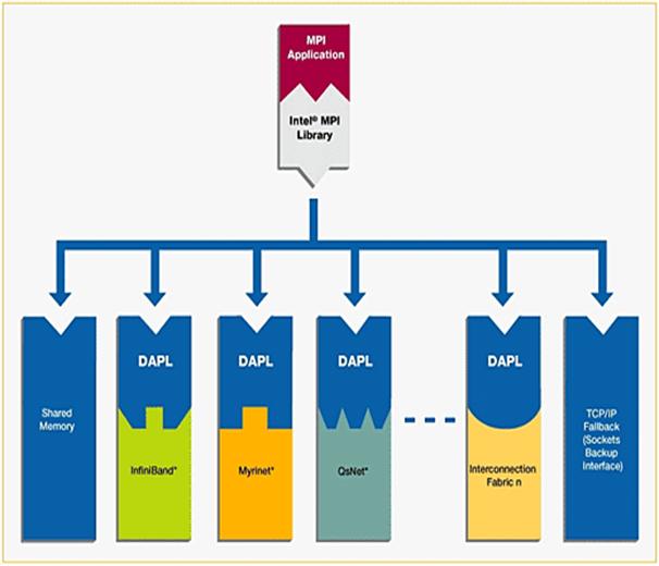
The software architecture for Intel MPI Library is described in Figure 4.1. With Intel MPI Library on Linux-based systems, you can choose the best interconnection fabric for running an application on a cluster that is based on IA-32, or Intel® 64 architecture. This is done at runtime by setting the I_MPI_FABRICS environment variable (See Section 4.4). Execution failure can be avoided even if interconnect selection fails. This is especially true for batch computing. For such situations, the sockets interface will automatically be selected (Figure 4.1) as a backup.
Similarly using Intel MPI Library on Microsoft Windows CCS* OS, you can choose the best interconnection fabric for running an application on a cluster that is based on Intel® 64 architecture.

4.1 Launching MPD Daemons
The Intel MPI Library uses a Multi-Purpose Daemon (MPD) job startup mechanism. In order to run programs compiled with mpicc (or related) commands, you must first set up MPD daemons. It is strongly recommended that you start and maintain your own set of MPD daemons, as opposed to having the system administrator start up the MPD daemons once for use by all users on the system. This setup enhances system security and gives you greater flexibility in controlling your execution environment.
4.2 How to Set Up MPD Daemons on Linux* OS
1. Set up environment variables with appropriate values and directories, e.g., in the .cshrc or .bashrc files. At a minimum, set the following environment variables: Ensure that the PATH variable includes the following:
· The <directory-path-to-Intel-MPI-Library>/bin directory. For example, the <directory-path-to-Intel-MPI-Library>/bin directory path should be set.
· Directory for Python* version 2.2 or greater.
· If you are using Intel® C++ and/or Intel® Fortran Compilers, ensure that the LD_LIBRARY_PATH variable contains the directories for the compiler library. You can set this variable by using the *vars.[c]sh scripts included with the compiler. Set any additional environment variables your application uses.
2. Create a $HOME/.mpd.conf file that contains your MPD password. Your MPD password is not the same as any Linux login password, but rather is used for MPD only. It is an arbitrary password string that is used only to control access to the MPD daemons by various cluster users. To set up your MPD password:
secretword=<your mpd secretword>
Do not use any Linux login password for <your mpd secretword>. An arbitrary <your mpd secretword> string only controls access to the MPD daemons by various cluster users.
3. Set protection on the file so that you have read and write privileges, for example, and ensure that the $HOME/.mpd.conf file is visible on, or copied to, all the nodes in the cluster as follows:
chmod 600 $HOME/.mpd.conf
4. Verify that PATH settings and .mpd.conf contents can be observed through rsh on all nodes in the cluster. For example, use the following commands with each <node> in the cluster:
rsh <node> env
rsh <node> cat $HOME/.mpd.conf
5. Create an mpd.hosts text file that lists the nodes in the cluster, with one machine name per line, for use by mpdboot. Recall that the contents of the machines.LINUX file that was referenced previously can be used to construct an mpd.hosts file.
6. Start up the MPD daemons as follows:
mpdboot [ -d -v ] -n <#nodes> [-f <path/name of mpd.hosts file>]
For more information about the mpdboot command, see Setting up MPD Daemons in the <directory-path-to-Intel-MPI-Library>/doc/Getting_Started.pdf or the mpdboot section of <directory-path-to-Intel-MPI-Library>/doc/Reference_Manual.pdf.
7. Determine the status of the MPD daemons as follows:
mpdtrace
The output should be a list of nodes that are currently running MPD daemons.
Remarks
- If required, shut down the MPD daemons as follows:
mpdallexit
- You as a user should start your own set of MPD daemons. It is not recommended to start MPD as root due to setup problems and security issues.
4.3 The mpdboot Command for Linux* OS
Use the mpdboot –f <hosts file> option to select a specific hosts file to be used. The default is to use ${PWD}/mpd.hosts. A valid host file must be accessible in order for mpdboot to succeed. As mentioned previously, the contents of the machines.LINUX file can also be used by you to construct an mpd.hosts file.
4.4 Compiling and Linking with Intel® MPI Library on Linux* OS
This section describes the basic steps required to compile and link an MPI program, when using only the Intel MPI Library Development Kit. To compile and link an MPI program with the Intel MPI Library:
1. Ensure that the underlying compiler and related software appear in your PATH. If you are using Intel compilers, insure that the compiler library directories appear in LD_LIBRARY_PATH environment variable. For example, regarding the Intel 11.1 compilers, execution of the appropriate set-up scripts will do this automatically (the build number for the compilers might be something different than “11.1/035” for your installation):
/opt/intel/Compiler/11.1/035/bin/iccvars.[c]sh
and
/opt/intel/Compiler/11.1/035/bin/ifortvars.[c]sh
2. Compile your MPI program via the appropriate mpi compiler command. For example, C code uses the mpiicc command as follows:
mpiicc <directory-path-to-Intel-MPI-Library>/test/test.c
Other supported compilers have an equivalent command that uses the prefix mpi on the standard compiler command. For example, the Intel MPI Library command for the Intel® Fortran Compiler (ifort) is mpiifort.
|
Supplier of Core Compiler |
MPI Compilation Command |
Core Compiler Compilation Command |
Compiler Programming Language |
Support Application Binary Interface (ABI) |
|
GNU* Compilers |
mpicc |
gcc, cc |
C |
32/64 bit |
|
mpicxx |
g++ version 3.x g++ version 4.x |
C/C++ |
32/64 bit |
|
|
mpif77 |
f77 or g77 |
Fortran 77 |
32/64 bit |
|
|
mpif90 |
gfortran |
Fortran 95 |
32/64 bit |
|
|
Intel C++ and Fortran Compilers versions 10.1, 11.0, or 11.1 |
mpiicc |
icc |
C |
32/64 bit |
|
mpiicpc |
icpc |
C++ |
32/64 bit |
|
|
mpiifort |
ifort |
Fortran 77 and Fortran 95 |
32/64 bit |
Remarks
The Compiling and Linking section of <directory-path-to-Intel-MPI-Library>/doc/Getting_Started.pdf or the Compiler Commands section of <directory-path-to-Intel-MPI-Library>/doc/Reference_Manual.pdf on the system where Intel MPI Library is installed include additional details on mpiicc and other compiler commands, including commands for other compilers and languages.
4.5 Selecting a Network Fabric
Intel MPI Library supports multiple, dynamically selectable network fabric device drivers to support different communication channels between MPI processes. The default communication method uses a built-in TCP (Ethernet, or sockets) device driver. Prior to the introduction of Intel® MPI Library 4.0, selection of alternative devices was done via the command line using the I_MPI_DEVICE environment variable. With Intel® MPI Library 4.0 and its successors, the I_MPI_FABRICS environment variable is to be used, and the environment variable I_MPI_DEVICE is considered a deprecated syntax. The following network fabric types for I_MPI_FABRICS are supported by Intel MPI Library 4.0 and its successors:
|
Possible Interconnection-Device-Fabric Values for the I_MPI_FABRICS Environment Variable |
Interconnection Device Fabric Meaning |
|
shm |
Shared-memory |
|
dapl |
DAPL–capable network fabrics, such as InfiniBand*, iWarp*, Dolphin*, and XPMEM* (through DAPL*) |
|
tcp |
TCP/IP-capable network fabrics, such as Ethernet and InfiniBand* (through IPoIB*) |
|
tmi |
Network fabrics with tag matching capabilities through the Tag Matching Interface (TMI), such as Qlogic* and Myrinet* |
|
ofa |
Network fabric, such as InfiniBand* (through OpenFabrics* Enterprise Distribution (OFED*) verbs) provided by the Open Fabrics Alliance* (OFA*) |
The environment variable I_MPI_FABRICS has the following syntax:
I_MPI_FABRICS=<fabric> | <intra-node fabric>:<internodes-fabric>
where the <fabric> value meta-symbol can have the values shm, dapl, tcp, tmi, or ofa. The <intra-node fabric> value meta-symbol can have the values shm, dapl, tcp, tmi, or ofa. Finally, the <inter-node fabric> value meta-symbol can have the values dapl, tcp, tmi, or ofa.
The next section will provide some examples for using the I_MPI_FABRICS environment variable within the mpiexec command-line.
4.6 Running an MPI Program Using Intel® MPI Library on Linux* OS
Use the mpiexec command to launch programs linked with the Intel MPI Library example:
mpiexec -n <# of processes> ./myprog
The only required option for the mpiexec command is the -n option to set the number of processes. If your MPI application is using a network fabric other than the default fabric, use the –env option to specify a value to be assigned to the I_MPI_FABRICS variable. For example, to run an MPI program while using the shared memory for intra-node communication and sockets for inter-node communication, use the following command:
mpiexec -n <# of processes> -env I_MPI_FABRICS shm:tcp ./myprog
As an example of running an MPI application on a cluster system with a combined shared-memory and DAPL-enabled network fabric, the following mpiexec command-line might be used:
mpiexec -n <# of processes> -env I_MPI_FABRICS shm:dapl ./myprog
See the section titled Selecting a Network Fabric in <directory-path-to-Intel-MPI-Library>/doc/Getting_Started.pdf, or the section titled Fabrics Control in <directory-path-to-Intel-MPI-Library>/doc/Reference_Manual.pdf.
4.7 Experimenting with Intel® MPI Library on Linux* OS
For the experiments that follow, it is assumed that a computing cluster has at least 2 nodes and there are two symmetric multi-processors (SMPs) per node. Start up the MPD daemons by issuing a command such as:
mpdboot -n 2 -r rsh -f ~/mpd.hosts
Type the command:
mpdtrace
to verify that there are MPD daemons running on the two nodes of the cluster. The response from issuing this command should be something like:
clusternode1
clusternode2
assuming that the two nodes of the cluster are called clusternode1 and clusternode2. The actual response will be a function of your cluster configuration.
In the <directory-path-to-Intel-MPI-Library>/test folder where Intel MPI Library resides, there are source files for four MPI test cases. In your local user area, you should create a test directory called:
test_intel_mpi/
From the installation directory of Intel MPI Library, copy the test files from <directory-path-to-Intel-MPI-Library>/test to the directory above. The contents of test_intel_mpi should now be:
test.c test.cpp test.f test.f90
Compile the test applications into executables using the following commands:
mpiifort test.f -o testf
mpiifort test.f90 -o testf90
mpiicc test.c -o testc
mpiicpc test.cpp -o testcpp
Issue the mpiexec commands:
mpiexec -n 2 ./testf
mpiexec -n 2 ./testf90
mpiexec -n 2 ./testc
mpiexec -n 2 ./testcpp
The output from testcpp should look something like:
Hello world: rank 0 of 2 running on clusternode1
Hello world: rank 1 of 2 running on clusternode2
If you have successfully run the above applications using Intel MPI Library, you can now run (without re-linking) the four executables on clusters that use Direct Access Program Library (DAPL) interfaces to alternative interconnection fabrics. If you encounter problems, please see the section titled Troubleshooting within the document Intel MPI Library Getting Started Guide located in <directory-path-to-Intel-MPI-Library>/doc/Getting_Started.pdf for possible solutions.
Assuming that you have a dapl device fabric installed on the cluster, you can issue the following commands for the four executables so as to access that device fabric:
mpiexec -env I_MPI_FABRICS dapl -n 2 ./testf
mpiexec -env I_MPI_FABRICS dapl -n 2 ./testf90
mpiexec –env I_MPI_FABRICS dapl -n 2 ./testc
mpiexec -env I_MPI_FABRICS dapl -n 2 ./testcpp
The output from testf90 using the dapl device value for the I_MPI_FABRICS environment variable should look something like:
Hello world: rank 0 of 2 running on
clusternode1
Hello world: rank 1 of 2 running on
clusternode2
4.8 Controlling MPI Process Placement on Linux* OS
The mpiexec command controls how the ranks of the processes are allocated to the nodes in the cluster. By default, mpiexec uses round-robin assignment of ranks to the nodes. This placement algorithm may not be the best choice for your application, particularly for clusters with SMP (symmetric multi-processor) nodes.
Suppose that the geometry is <#ranks> = 4 and <#nodes> = 2, where adjacent pairs of ranks are assigned to each node (for example, for 2-way SMP nodes). Issue the command:
cat ~/mpd.hosts
The results should be something like:
clusternode1
clusternode2
Since each node of the cluster is a 2-way SMP, and 4 processes are to be used for the application, the next experiment will distribute the 4 processes such that 2 of the processes will execute on clusternode1 and 2 will execute on clusternode2. For example, you might issue the following commands:
mpiexec -n 2 -host clusternode1 ./testf : -n 2 -host clusternode2 ./testf
mpiexec -n 2 -host clusternode1 ./testf90 : -n 2 -host clusternode2 ./testf90
mpiexec -n 2 -host clusternode1 ./testc : -n 2 -host clusternode2 ./testc
mpiexec -n 2 -host clusternode1 ./testcpp : -n 2 -host clusternode2 ./testcpp
The following output should be produced for the executable testc:
Hello world: rank 0 of 4 running on clusternode1
Hello world: rank 1 of 4 running on clusternode1
Hello world: rank 2 of 4 running on clusternode2
Hello world: rank 3 of 4 running on clusternode2
In general, if there are i nodes in the cluster and each node is j-way SMP system, then the mpiexec command-line syntax for distributing the i by j processes amongst the i by j processors within the cluster is:
mpiexec -n j -host <nodename-1> ./mpi_example : \
-n j -host <nodename-2> ./mpi_example : \
-n j -host <nodename-3> ./mpi_example : \
…
-n j -host <nodename-i> ./mpi_example
Note that you would have to fill in appropriate host names for <nodename-1> through <nodename-i> with respect to your cluster system. For a complete discussion on how to control process placement through the mpiexec command, see the Local Options section of the Intel MPI Library Reference Manual located in <directory-path-to-Intel-MPI-Library>/doc/Reference_Manual.pdf.
4.9 Using the Automatic Tuning Utility Called mpitune
The mpitune utility was first introduced with Intel® MPI Library 3.2. It can be used to find optimal settings of Intel® MPI Library in regards to the cluster configuration or a user’s application for that cluster.
As an example, the executables testc, testcpp, testf, and testf90 in the directory test_intel_mpi could be used. The command invocation for mpitune might look something like the following:
mpitune –-host-file machines.LINUX –-output-file testc.conf --application \”mpiexec –n 4 testc\”
where the options above are just a subset of the following complete command-line switches:
|
Command-line Option |
Semantic Meaning |
|
-a \”<app_cmd_line>\” | --application \”<app_cmd_line>\” |
Switch on the application tuning mode. Quote the full command line as shown |
|
-cm | --cluster-mode {exclusive | full} |
Set the cluster usage mode exclusive – only one task will executed on the cluster at a time full – maximum number of tasks will be execute. This is the default mode |
|
-d | --debug |
Print debug information |
|
-dl [d1[,d2…[,dN]]] | --device-list [d1[,d2…[,dN]]] |
Select the device(s) you want to tune. By default use all of the devices mentioned in the <installdir>/<arch>/etc/devices.xml file |
|
-er | --existing-ring |
Try to use an existing MPD ring. By default, create a new MPD ring |
|
-fl [f1[,f2…[,fN]]] | --fabric-list [f1[,f2…[,fN]]] |
Select the fabric(s) you want to tune. By default use all of the fabrics mentioned in the <installdir>/<arch>/etc/fabrics.xml file |
|
-h | --help |
Display a help message |
|
-hf <hostsfile> | --host-file <hostsfile> |
Specify an alternative host file name. By default, use the $PWD/mpd.hosts |
|
-hr | --host-range {min:max | min: | :max} |
Set the range of hosts used for testing. The default minimum value is 1. The default maximum value is the number of hosts defined by the mpd.hosts or the existing MPD ring. The min: or :max format will use the default values as appropriate |
|
-i <count> | --iterations <count> |
Define how many times to run each tuning step. Higher iteration counts increase the tuning time, but may also increase the accuracy of the results. The default value is 3 |
|
-mh | --master-host |
Dedicate a single host to mpitune |
|
--message-range {min:max | min: | :max} |
Set the message size range. The default minimum value is 0. The default maximum value is 4194304 (4mb). By default, the values are given in bytes. They can also be given in the following format: 16kb, 8mb, or 2gb. The min: or :max format will use the default values as appropriate |
|
-of <file-name> | --output-file <file-name> |
Specify the application configuration file to be generated in the application-specific mode. By default, use the $PWD/app.conf |
|
-od <outputdir> | --output-directory <outputdir> |
Specify the directory name for all output files. By default, use the current directory. The directory should be accessible from all hosts |
|
-pr {min:max | min: | :max} | -–ppn-range {min:max | min: | :max} | -–perhost-range {min:max | min: | :max} |
Set the maximum number of processes per host. The default minimum value is 1. The default maximum value is the number of cores of the processor. The min: or :max format will use the default values as appropriate |
|
-sf [file-path] | --session-file [file-path] |
Continue the tuning process starting from the state saved in the file-path session file |
|
-s | --silent |
Suppress all diagnostic output |
|
-td <dir-path> | --temp-directory <dir-path> |
Specify a directory name for the temporary data. By default, use the $PWD/mpitunertemp. This directory should be accessible from all hosts |
|
-t \”<test_cmd_line>\” | --test \”<test_cmd_line>\” |
Replace the default Intel® MPI Benchmarks by the indicated benchmarking program in the cluster-specific mode. Quote the full command line as shown |
|
-tl <minutes> | --time-limit <minutes> |
Set mpitune execution time limit in minutes. The default value is 0, which means no limitations |
|
-V | --version |
Print out the version information |
Details on optimizing the settings for Intel® MPI Library with regards to the cluster configuration or a user’s application for that cluster are described in the next two subsections.
4.9.1 Cluster Specific Tuning
Once you have installed the Intel® Cluster Tools on your system you may want to use the mpitune utility to generate a configuration file that is targeted at optimizing the Intel® MPI Library with regards to the cluster configuration. For example, the mpitune command:
mpitune –hf machines.LINUX –of testc.conf –-test \”testc\”
could be used, where machines.LINUX contains a list of the nodes in the cluster. Completion of this command may take some time. The mpitune utility will generate a configuration file that might have a name such as app.conf. You can then proceed to run the mpiexec command on an application using the –tune option. For example, the mpiexec command-line syntax for the testc executable might look something like the following:
mpiexec –tune –n 4 testc
4.9.2 MPI Application-Specific Tuning
The mpitune invocation:
mpitune –hf machines.Linux –of testf90.conf --application \”mpiexec –n 4 testf90\”
will generate a file called app.config that is base on the application testf90. Completion of this command may take some time also. This configuration file can be used in the following manner:
mpiexec –tune testf90.conf –n 4 testf90
where the mpiexec command will load the configuration options recorded in testf90.conf.
You might want to use mpitune utility on each of the test applications testc, testcpp, testf, and testf90. For a complete discussion on how to use the mpitune utility, see the Tuning Reference section of the Intel MPI Library for Linux* OS Reference Manual located in <directory-path-to-Intel-MPI-Library>/doc/Reference_Manual.pdf.
4.10 Extended File I/O System Support on Linux* OS
Intel® MPI Library provides loadable shared library modules to provide native support for the following file I/O systems:
· Panasas* ActiveScale* File System (PanFS)
· Parallel Virtual File System*, Version 2 (Pvfs2)
Set the I_MPI_EXTRA_FILESYSTEM environment variable to on to enable parallel file system support. Set the I_MPI_EXTRA_FILESYSTEM_LIST environment variable to request native support for the specific file system. For example, to request native support for the Panasas* ActiveScale* File System, do the following:
mpiexec –env I_MPI_EXTRA_FILESYSTEM on –env I_MPI_EXTRA_FILESYSTEM_LIST panfs –n 4 ./myprog
4.10.1 How to Use the Environment Variables I_MPI_EXTRA_FILESYSTEM and I_MPI_EXTRA_FILESYSTEM_LIST
The environment variable I_MPI_EXTRA_FILESYSTEM is used to enable parallel I/O file system support. The general syntax for this environment variable is:
I_MPI_EXTRA_FILESYSTEM=<value>
where <value> can be:
|
Value |
Meaning |
|
enable or yes or on or 1 |
Turn on native support for a parallel file I/O system |
|
disable or no or off or 0 |
Turn off native support for a parallel file I/O system. This is the default setting. |
In conjunction with the I_MPI_EXTRA_FILESYSTEM environment variable, the environment variable I_MPI_EXTRA_FILESYSTEM_LIST will control which file I/O system or systems are used. In general, the syntax for the I_MPI_EXTRA_FILESYSTEM_LIST environment variable is:
I_MPI_EXTRA_FILESYSTEM_LIST=<file-system1>[,<file-system2>,<file-system3>, … , <file-systemn>]
where <file-systemi> can be:
|
File I/O System <file-systemi> |
Meaning |
|
panfs |
Panasas* ActiveScale* File system |
|
Pvfs2 |
Parallel Virtual File System, Version 2 |
The mpiexec and mpirun commands associated with Intel® MPI Library will load the shared I/O libraries associated with the I_MPI_EXTRA_FILESYSTEM_LIST environment variable. As mentioned previously, the environment variables I_MPI_EXTRA_FILESYSTEM and I_MPI_EXTRA_FILESYSTEM_LIST must be used together.
For a complete discussion on how to use the environment variables I_MPI_EXTRA_FILESYSTEM and I_MPI_EXTRA_FILESYSTEM_LIST, see the Extended File System Support section of the Intel MPI Library for Linux* OS Reference Manual located in <directory-path-to-Intel-MPI-Library>/doc/Reference_Manual.pdf.
To make inquiries about Intel MPI Library, visit the URL: http://premier.intel.com.
As mentioned previously (e.g., Figure 2.1), components of the Intel Cluster Toolkit Compiler Edition will now work with the Intel Debugger. The Intel Debugger is a parallel debugger with the following software architecture (Figure 5.1):
Figure 5.1 – The Software Architecture of the Intel Debugger
With respect to Figure 5.1, there is a user interface to a root debugger. This is demonstrated at the bottom of Figure 5.1. The root debugger communicates with a tree of parallel debuggers. These are the leaf nodes at the top of the illustration. There are aggregation capabilities for consolidating debug information. This is done through the aggregators in Figure 5.1.
All processes with the same output are aggregated into a single and final output message. As an example, the following message represents 42 MPI processes:
[0-41] Linux Application Debugger for Xeon(R)-based applications, Version XX
Diagnostics which have different hexadecimal digits, but are otherwise identical, are condensed by aggregating the differing digits into a range. As an example:
[0-41]>2 0x120006d6c in feedback(myid=[0;41],np=42,name=0x11fffe018="mytest") "mytest.c":41
5.1 Login Session Preparations for Using Intel® Debugger on Linux* OS
The debugger executable for the Intel Debugger is called idb. In the 11.1 version of the Intel® Debugger, the idb command invokes the GUI. Alternatively for the 11.1 version of Intel® Debugger, to get the command-line interface, use idbc. There are three steps that should be followed in preparing your login session so that you can use the Intel Debugger.
1. The Intel® IDB Debugger graphical environment is a Java application and requires a Java* Runtime Environment* (JRE*) to execute. The debugger will run with a version 5.0 (also called 1.5) JRE.
Install the JRE according to the JRE provider's instructions.
Finally you need to export the path to the JRE as follows:
export PATH=<path_to_JRE_bin_DIR>:$PATH export
2. Set the environment variable IDB_HOME to the folder path where the Intel Debugger executable, idb, resides. Also, you will want to source either idbvars.sh or idbvars.csh through ifortvars.[c]sh or iccvars.[c]sh depending on which command-line shell you are using. For example in augmenting your .bashrc file for the Bourne Shell or the Korn Shell, you can source the Intel® Compiler Pro C++ file called iccvars.sh or the Intel® Compiler Pro Fortran file ifortvars.sh which are located within the bin directory of the Intel® Compiler Pro installation directory on your system. Regarding your .bashrc file, the Bourne Shell or the Korn Shell sourcing syntax might look something like the following for Intel® 64 architecture:
. /opt/intel/Compiler/11.1/060/bin/iccvars.sh intel64
export IDB_HOME=/opt/intel/Compiler/11.1/060/bin/intel64
or
. /opt/intel/Compiler/11.1/060/bin/ifortvars.sh intel64
export IDB_HOME=/opt/intel/Compiler/11.1/060/bin/intel64
For augmenting your .cshrc file, the C Shell syntax should be something like:
source /opt/intel/Compiler/11.1/060/bin/iccvars.csh intel64
setenv IDB_HOME /opt/intel/Compiler/11.1/060/bin/intel64
or
source /opt/intel/Compiler/11.1/060/bin/ifortvars.csh intel64
setenv IDB_HOME /opt/intel/Compiler/11.1/060/bin/intel64
Depending on the Intel® architecture, the argument to iccvars.[c]sh and ifortvars.[c]sh can be ia32, or intel64. Sourcing iccvars.[c]sh or ifortvars.[c]sh will update the PATH and MANPATH environment variables also.
3. Edit the ~/.rhosts file in your home directory so that it contains the list of nodes that comprise the cluster. Recall that previously we referred to the contents of a file called machines.LINUX, where a contrived cluster consisting of eight nodes might be:
clusternode1
clusternode2
clusternode3
clusternode4
clusternode4
clusternode6
clusternode7
clusternode8
For example, assuming that the names listed above make up your cluster, they could be added to your ~/.rhosts file with the following general syntax:
<hostname as echoed by the shell command hostname> <your username>
For the list of nodes above and assuming that your login name is user01, the contents of your ~/.rhosts file might be:
clusternode1 user01
clusternode2 user01
clusternode3 user01
clusternode4 user01
clusternode5 user01
clusternode6 user01
clusternode7 user01
clusternode8 user01
The permission bit settings of ~/.rhosts should be set to 600 using the chmod command. The shell command for doing this might be:
chmod 600 ~/.rhosts
Once the three steps above are completed, you are ready to use the Intel Debugger. The general syntax for using the Intel Debugger with Intel MPI Library is as follows:
mpiexec -idb –genv MPIEXEC_DEBUG 1 -n <number of processes> [other Intel MPI options] <executable> [arguments to the executable]
The environment variable MPIEXEC_DEBUG needs to be referenced so that MPI processes will suspend their execution to wait for the debuggers to attach to them. For the command-line example above, the –genv command-line option sets the environment variable MPIEXEC_DEBUG for all MPI processes. In general, the global environment variable command line switch –genv has the syntax:
–genv <environment variable> <value>
where <environment variable> is a meta-symbol that is a stand-in for a relevant environment variable, and <value> is a stand-in for setting an appropriate value for the preceding environment variable name.
For the contents of the directory test_intel_mpi that was described in Chapter 4, there should be the four source files:
test.c test.cpp test.f test.f90
Compile the test applications into executables using the following commands:
mpiifort –g test.f -o testf
mpiifort –g test.f90 -o testf90
mpiicc –g test.c -o testc
mpiicpc –g test.cpp -o testcpp
You can issue mpiexec commands that might look something like the following:
mpiexec –idb –genv MPIEXEC_DEBUG 1 -n 4 ./testf
mpiexec –idb –genv MPIEXEC_DEBUG 1 -n 4 ./testf90
mpiexec –idb –genv MPIEXEC_DEBUG 1 -n 4 ./testc
mpiexec –idb –genv MPIEXEC_DEBUG 1 -n 4 ./testcpp
The commands above are using four MPI processes. Figure 5.2 shows what the debug session might look like after issuing the shell command:
mpiexec –idb –genv MPIEXEC_DEBUG 1 -n 4 ./testcpp
In Figure 5.2, the debugger stops the testcpp application at the C++ method MPI::Init(argc, argv).
Figure 5.2 – idb session for the executable called testc
Note: The user interface for idb is gdb*-compatible by default. To see where the MPI application is with respect to execution, you can type the IDB command called where after the prompt (idb) in Figure 5.2. This will produce a call stack something like what is shown in Figure 5.3.
Figure 5.3 – The application call stack after typing the IDB command where
Recall that the C++ application has the source file name test.cpp and according to the IDB debugger stack trace, the line referenced in test.cpp is line 29. If you would like to use a text editor to look at test.cpp, you can modify the debugging user interface from the default which is gdb* to that if idb by typing the debug command:
set $cmdset = "idb"
You can then type the command:
edit +29 test.cpp
in Figure 5.3 and the result will be something like that shown in Figure 5.4. Line 29 of test.cpp is the MPI library call to Init. The edit session in Figure 5.4 is using the vi editor. In general, the editor that is invoked is a function of the EDITOR environment variable.
Figure 5.4 – Launching of an edit session from the Intel Debugger
You can use the command :q! to close the vi edit session. This is demonstrated in Figure 5.5.
Figure 5.5 – Terminating the vi editing session using the command :q!
The "run" command is disabled in MPI debugging. To continue the execution of the MPI application, use “cont”. If you proceed to type the word cont after the (idb) prompt shown at the bottom of Figure 5.6, then debugging session results that might look something like that shown in Figure 5.7 will appear. Also, “Hello world” messages will appear in the login session where the mpiexec command was issued.
Figure 5.6 – Returning control back to IDB after terminating the editing session
The 4 MPI processes for the example in Figure 5.7 are labeled 0 to 3.
Figure 5.7 – State of the IDB session as a result of issuing the IDB command cont
You can type the word quit to end the IDB debug session, and therefore close the display shown in Figure 5.7.
Unfortunately, the rerun command is not yet supported within IDB. To rerun MPI application with the IDB debugger, you will have to quit IDB and then re-enter the mpiexec command.
For a complete discussion on how to use the Intel Debugger (9.1.x or greater) please review the contents of the Intel Debugger (IDB) Manual located in <directory-path-to-Intel-Debugger>/doc/Doc_Index.htm on your computing system.
To make inquiries about the Intel Debugger, visit the URL: http://premier.intel.com.
In the folder path where Intel Trace Analyzer and Collector reside, there is a folder called examples. The folder path where the examples directory resides might be something like:
/opt/intel/ictce/4.0.0.017/itac/examples
If you copy the examples folder into a work area which is accessible by all of the nodes of the cluster, you might try the following sequence of commands:
gmake distclean
gmake all
This set of commands will respectively clean up the folder content and compile and execute the following C and Fortran executables:
vnallpair
vnallpairc
vnjacobic
vnjacobif
vtallpair
vtallpairc
vtcounterscopec
vtjacobic
vtjacobif
If you select the executable vtjacobic and run it with the following environment variable setting:
setenv VT_LOGFILE_PREFIX vtjacobic_inst
where the mpiexec command uses 4 processes as shown:
mpiexec -n 4 ./vtjacobic
then the trace data will be placed into the folder vtjacobic_inst. The contents of vtjacobic_inst will look something like the following:
. vtjacobic.stf.dcl vtjacobic.stf.msg.anc
.. vtjacobic.stf.frm vtjacobic.stf.pr.0
vtjacobic.prot vtjacobic.stf.gop vtjacobic.stf.pr.0.anc
vtjacobic.stf vtjacobic.stf.gop.anc vtjacobic.stf.sts
vtjacobic.stf.cache vtjacobic.stf.msg
when the command:
ls –aC --width=80 vtjacobic_inst
is used. If you run the Intel Trace Analyzer with the command:
traceanalyzer vtjacobic_inst/vtjacobic.stf
the following display panel will appear (Figure 6.1):
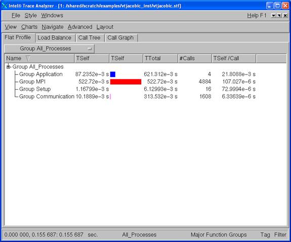
Figure 6.1 - Intel Trace Analyzer Display for vtjacobic.stf
Figure 6.2 shows the Event Timeline display which results when following the menu path Charts->Event Timeline within Figure 6.1.
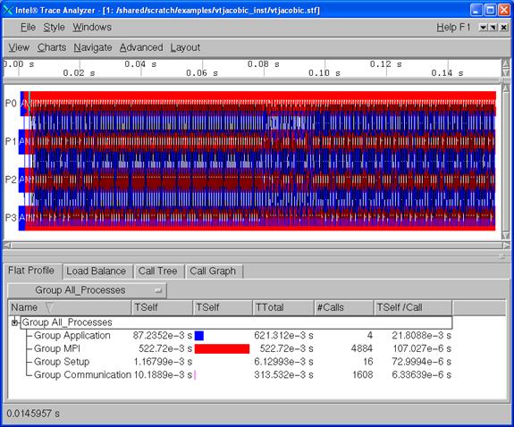
Figure 6.2 - Intel Trace Analyzer Display for vtjacobic.stf using Charts->Event Timeline
You can use the trace analyzer to view the contents of the other *.stf files in this working directory on your cluster system.
6.1 Experimenting with Intel® Trace Analyzer and Collector in a Fail-Safe Mode
There may be situations where an application will end prematurely, and thus trace data could be lost. The Intel Trace Collector has a trace library that works in fail-safe mode. An example shell command-line syntax for linking such a library is:
mpiicc test.c -o testc_fs -L${VT_LIB_DIR} -lVTfs ${VT_ADD_LIBS}
where the special Intel Trace Collector Library for fail-safe (acronym fs) tracing is –lVTfs.
In case of execution failure by the application, the fail-safe library freezes all MPI processes and then writes out the trace file. Figure 6.3 shows an Intel Trace Analyzer display for test.c.
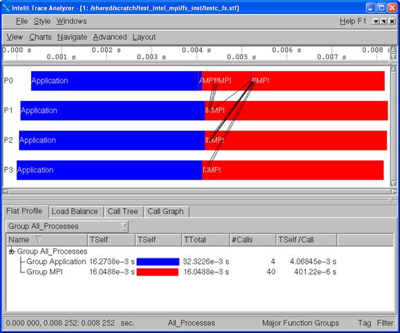
Figure 6.3 – Intel Trace Analyzer display of Fail-Safe Trace Collection by Intel Trace Collector
Complete user documentation regarding -lVTfs for the Intel Trace Collector can be found within the file:
<directory-path-to-ITAC>/doc/ITC_Reference_Guide.pdf
on the system where the Intel Trace Collector is installed. You can use vtfs as a search phrase within the documentation.
6.2 Using itcpin to Instrument an Application
The itcpin utility is a binary instrumentation tool that comes with Intel Trace Analyzer and Collector. The Intel® architectures must be IA-32, and Intel® 64.
The basic syntax for instrumenting a binary executable with the itcpin utility is as follows:
itcpin [<ITC options>] -- <application command line>
where -- is a delimiter between Intel Trace Collector (ITC) options and the application command-line.
The <ITC options> that will be used here is:
--run (off)
itcpin only runs the given executable if this option is used.
Otherwise it just analyzes the executable and prints configurable
information about it.
--insert
Intel Trace Collector has several libraries that can be used to do different kinds of tracing. An example library value could be VT which is the Intel Trace Collector Library. This is the default instrumentation library.
To obtain a list of all of the itcpin options simply type:
itcpin -–help
To demonstrate the use of itcpin, you can compile a C programming language example for calculating the value of “pi” where the application uses the MPI parallel programming paradigm. You can download the C source from the URL:
http://www.nccs.gov/wp-content/training/mpi-examples/C/pical.c
For the pi.c example, the following shell commands will allow you to instrument the binary called pi.exe with Intel Trace Collector instrumentation. The shell commands before and after the invocation of itcpin should be thought of as prolog and epilog code to aid in the use of the itcpin utility.
mpiicc -o pi.exe pi.c
setenv VT_LOGFILE_FORMAT STF
setenv VT_PCTRACE 5
setenv VT_LOGFILE_PREFIX ${PWD}/itcpin_inst
setenv VT_PROCESS "0:N ON"
rm -rf ${VT_LOGFILE_PREFIX}
mkdir ${VT_LOGFILE_PREFIX}
mpiexec –n 4 itcpin --run -- pi.exe
The shell commands above could be packaged into a C Shell script. An explanation for the instrumentation environment variables can be found in the Intel Trace Collector Users’ Guide under the search topic “ITC Configuration”.
The output from the above sequence or C Shell commands looks something like the following:
Process 0 of 4 on cluster01
Process 1 of 4 on cluster02
Process 3 of 4 on cluster03
Process 2 of 4 on cluster04
pi is approximately 3.1415926544231239, Error is 0.0000000008333307
wall clock time = 0.000427
[0] Intel(R) Trace Collector INFO: Writing tracefile pi.exe.stf in /shared/scratch/itcinstrument/itcpin_inst
Figure 6.4 shows the timeline and function panel displays that were generated from the instrumentation data that was stored into the directory ${PWD}/itcpin_inst as indicated by the environment variable VT_LOGFILE_PREFIX. The command that initiated the Intel Trace Analyzer with respect to the directory ${PWD} was:
traceanalyzer itcpin_inst/pi.exe.stf &
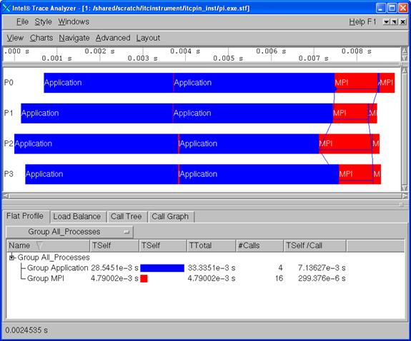
Figure 6.4 – Intel Trace Analyzer display of the “pi” integration application that has been binary instrumented with itcpin
Complete user documentation regarding itcpin for the Intel Trace Collector can be found within the file:
<directory-path-to-ITAC>/doc/ITC_Reference_Guide.pdf
on the system where the Intel Trace Collector is installed. You can use itcpin as a search phrase within the documentation. To make inquiries about the Intel Trace Analyzer, visit the URL: http://premier.intel.com.
6.3 Experimenting with Intel® Trace Analyzer and Collector in Conjunction with the LD_PRELOAD Environment Variable
There is an environment variable called LD_PRELOAD which can be initialized to reference instrumentation libraries. LD_PRELOAD instructs the operating system loader to load additional libraries into a program, beyond what was specified when it was initially compiled. In general, this environment variable allows users to add or replace functionality such as inserting performance tuning instrumentation. For Bourne* Shell or Korn* Shell the syntax for setting the LD_PRELOAD environment variable to instrument with Intel Trace Collector might be:
export LD_PRELOAD="libVT.so:libdl.so"
For C Shell, the syntax might be:
setenv LD_PRELOAD "libVT.so:libdl.so"
For the pi.c example, the following shell commands will allow you to use the LD_PRELOAD environment variable to instrument a binary with Intel Trace Collector instrumentation.
mpiicc -o pi.exe pi.c
setenv VT_PCTRACE 5
setenv VT_LOGFILE_PREFIX ${PWD}/ld_preload_inst
setenv VT_PROCESS "0:N ON"
setenv LD_PRELOAD "libVT.so:libdl.so"
rm -rf ${VT_LOGFILE_PREFIX}
mkdir ${VT_LOGFILE_PREFIX}
mpiexec -n 4 ./pi.exe 1000000
As mentioned previously, the shell commands above could be packaged into a C Shell script. The mpiexec command uses 4 MPI processes and the value of 1,000,000 indicates the number of intervals that will be used in the calculation of “pi”. Figure 6.5 shows the timeline and function panel displays that were generated from the instrumentation data that was stored in the directory ${PWD}/ld_preload_inst as indicated by the environment variable VT_LOGFILE_PREFIX. The command that initiated the Intel Trace Analyzer with respect to the directory ${PWD} was:
traceanalyzer ld_preload_inst/pi.exe.instr.stf &
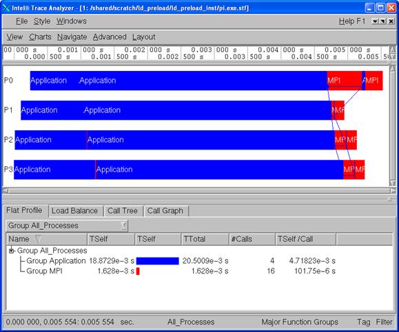
Figure 6.5 – Intel Trace Analyzer display of the “pi” integration application that has been instrumented through the LD_PRELOAD environment variable
Complete user documentation regarding LD_PRELOAD for the Intel Trace Collector can be found within the file:
<directory-path-to-ITAC>/doc/ITC_Reference_Guide.pdf
on the system where the Intel Trace Collector is installed. You can use LD_PRELOAD as a search phrase within the documentation. To make inquiries about LD_PRELOAD in conjunction with Intel Trace Analyzer and Collector, visit the URL: http://premier.intel.com.
6.4 Experimenting with Intel® Trace Analyzer and Collector in Conjunction with PAPI* Counters
The counter analysis discussion that follows assumes that a PAPI library is installed on the cluster system. PAPI is an acronym for Performance API and it serves to gather information regarding performance counter hardware. Details can be found at the URL:
This discussion assumes that the PAPI library is installed in a directory path such as /usr/local/papi. In the examples directory for Intel Trace Analyzer and Collector, there is a subfolder called poisson. Using root privileges, the library called libVTsample.a needs to be configured in the lib directory of Intel Trace Analyzer and Collector so that PAPI instrumentation can be captured through the Intel Trace Analyzer and Collector. The library path for the Intel Trace Analyzer and Collector might be something like:
${VT_ROOT}/lib
In this directory, a system administrator can use the following gmake command to create the libVTsample.a library:
export PAPI_ROOT=/usr/local
gmake all
The environment variable PAPI_ROOT is used by the makefile to formulate the path to ${PAPI_ROOT}/include which is a directory that contains PAPI header files. When the libVTsample.a library is built, the Poisson example can be linked with PAPI instrumentation as follows:
gmake MPI_HOME=${I_MPI_ROOT} make_dir=./ LIB_PATH="" LIBS="-L${VT_ROOT}/lib –lVTsample –lVT –L${PAPI_ROOT}/papi/lib –lpapi ${VT_ADD_LIBS}"
The shell commands for running the poisson application might be the following:
rm -rf ${PWD}/papi_inst
mkdir ${PWD}/papi_inst
setenv LD_LIBRARY_PATH ${LD_LIBRARY_PATH}:${PAPI_ROOT}/papi/lib
setenv VT_LOGFILE_PREFIX ${PWD}/papi_inst
setenv VT_CONFIG ${PWD}/vtconfig
mpiexec -n 16 ./poisson
The Intel Trace Collector configuration file which is called vtconfig for the above example contains the following PAPI counter selection:
COUNTER PAPI_L1_DCM ON
This PAPI counter directive is for L1 data cache misses. The general syntax for counter directives is:
COUNTER <name of counter> ON
The value of ON indicates that this particular hardware counter is to be monitored by Intel Trace Collector. The names of the PAPI hardware counters can be found in the folder path ${PAPI_ROOT}/include/papiStdEventDefs.h on the system where the PAPI library is installed.
Figure 6.6 illustrates a maximized view for the Counter Timeline Chart and the Function Profile Chart that were generated from the instrumentation data that was stored in the directory ${PWD}/papi_inst as indicated by the environment variable VT_LOGFILE_PREFIX. The command that initiated the Intel Trace Analyzer with respect to the directory ${PWD} was:
traceanalyzer papi_inst/poisson.stf &
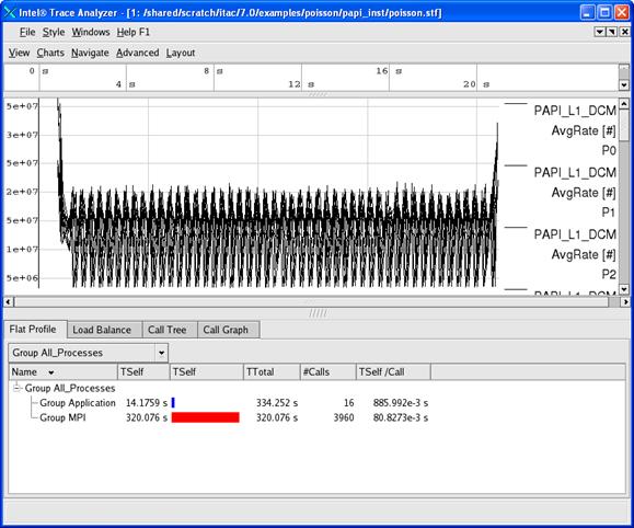
Figure 6.6 – A maximized view for the Counter Timeline Chart and the Function Profile Chart
Notice in the Counter Timeline Chart in Figure 6.6 that the PAPI counter PAPI_L1_DCM appears as a label in the right margin.
In general, the shell syntax for compiling the Intel MPI Library test files called test.c, test.cpp, test.f, and test.f90 with the PAPI interface involves the link options that look something like:
-L${VT_LIB_DIR} -lVTsample -lVT –L${PAPI_ROOT}/papi/lib -lpapi ${VT_ADD_LIBS}
The compilation commands are:
mpiicc test.c -o testc -L${VT_LIB_DIR} -lVTsample -lVT –L${PAPI_ROOT}/papi/lib -lpapi ${VT_ADD_LIBS}
mpiicpc test.cpp -o testcpp -L${VT_LIB_DIR} -lVTsample -lVT -L${PAPI_ROOT}/papi/lib -lpapi ${VT_ADD_LIBS}
mpiifort test.f -o testf -L${VT_LIB_DIR} -lVTsample -lVT -L${PAPI_ROOT}/papi/lib -lpapi ${VT_ADD_LIBS}
mpiifort test.f90 -o testf90 -L${VT_LIB_DIR} -lVTsample -lVT -L${PAPI_ROOT}/papi/lib -lpapi ${VT_ADD_LIBS}
On Linux, complete user documentation regarding PAPI hardware counters for the Intel Trace Collector can be found within the file:
<directory-path-to-ITAC>/doc/ITC_Reference_Guide.pdf
on the system where the Intel Trace Collector is installed. You can use PAPI as a search phrase within the documentation. To make inquiries about PAPI in conjunction with the Intel Trace Analyzer and Collector, visit the URL: http://premier.intel.com.
6.5 Experimenting with the Message Checking Component of Intel® Trace Collector
Intel Trace Collector environment variables which should be useful for message checking are:
VT_DEADLOCK_TIMEOUT <delay>, where <delay> is a time value. The default value is 1 minute and the notation for the meta-symbol <delay> could be 1m. This controls the same mechanism to detect deadlocks as in libVTfs which is the fail-safe library. For interactive use it is recommended to set it to a small value like “10s” to detect deadlocks quickly without having to wait long for the timeout.
VT_DEADLOCK_WARNING <delay> where <delay> is a time value. The default value is 5 minutes and the notation for the meta-symbol <delay> could be 5m. If on average the MPI processes are stuck in their last MPI call for more than this threshold, then a GLOBAL:DEADLOCK:NO PROGRESS warning is generated. This is a sign of a load imbalance or a deadlock which cannot be detected because at least one process polls for progress instead of blocking inside an MPI call.
VT_CHECK_TRACING <on | off>. By default, during correctness checking with libVTmc no events are recorded and no trace file is written. This option enables recording of all events also supported by the normal libVT and the writing of a trace file. The trace file will also contain the errors found during the run.
On Linux, complete user documentation regarding message checking for the Intel Trace Collector can be found within the file:
<directory-path-to-ITAC>/doc/ITC_Reference_Guide.pdf
The chapter title is called “Correctness Checking”.
An MPI application can be instrumented in four ways with the message checking library.
1) Compile the application with a static version of the message checking library:
mpiicc deadlock.c -o deadlock_static.exe -g -L ${VT_LIB_DIR} -lVTmc ${VT_ADD_LIBS}
mpiexec -genv VT_CHECK_TRACING on -genv VT_DEADLOCK_TIMEOUT 20s -genv VT_DEADLOCK_WARNING 25s -n 2 ./deadlock_static.exe 0 80000
2) Compile the application with a shared object version of the message checking library:
mpiicc deadlock.c -o deadlock_shared.exe -g -L ${VT_SLIB_DIR} -lVTmc ${VT_ADD_LIBS}
mpiexec -genv VT_CHECK_TRACING on -genv VT_DEADLOCK_TIMEOUT 20s -genv VT_DEADLOCK_WARNING 25s -n 2 ./deadlock_shared.exe 0 80000
Note that the library path for the Intel® C++ Compiler will vary from version to version.
3) Use the itcpin command:
mpiicc deadlock.c -o deadlock.exe –g
mpiexec -genv VT_CHECK_TRACING on -genv VT_DEADLOCK_TIMEOUT 20s -genv VT_DEADLOCK_WARNING 25s –n 2 itcpin --insert libVTmc.so -–run -- ./deadlock.exe 0 80000
4) Use the LD_PRELOAD environment variable with the mpiexec command. An example might be:
mpiicc deadlock.c -o deadlock.exe –g
mpiexec -genv VT_CHECK_TRACING on -genv LD_PRELOAD libVTmc.so -genv VT_DEADLOCK_TIMEOUT 20s -genv VT_DEADLOCK_WARNING 25s -n 2 ./deadlock.exe 0 80000
There is a sub-directory of the examples directory called checking. The checking directory has the following contents:
global/ GNUmakefile local/ misc/
The GNUmakefile has targets all, clean, print, and run, where all is the default. After type gmake, one can type the command:
gmake run
The output error diagnostics for the command above will be sent to stderr. If you wish to retain the output into a file, the results for stderr can be directed to a file.
Each leaf sub-folder contains a source file and an “*.ref.out” file which can be used as a point of reference for the expected diagnostics that the message checking component of the Intel® Trace Collector should capture. For example, if you search the global sub-directory, you will find a folder path of the following form:
global/collective/datatype_mismatch/
The contents of the leaf directory consist of:
MPI_Bcast.c MPI_Bcast.ref.out
The file MPI_Bcast.ref.out has diagnostic information that looks something like the following:
…
[0] INFO: initialization completed successfully
[0] ERROR: GLOBAL:COLLECTIVE:DATATYPE:MISMATCH: error
[0] ERROR: Mismatch found in local rank [1] (global rank [1]),
[0] ERROR: other processes may also be affected.
[0] ERROR: No problem found in local rank [0] (same as global rank):
[0] ERROR: MPI_Bcast(*buffer=0x7fbfffe9f0, count=1, datatype=MPI_INT, root=0, comm=MPI_COMM_WORLD)
[0] ERROR: main (global/collective/datatype_mismatch/MPI_Bcast.c:50)
[0] ERROR: 1 elements transferred by peer but 4 expected by
[0] ERROR: the 3 processes with local ranks [1:3] (same as global ranks):
[0] ERROR: MPI_Bcast(*buffer=0x7fbfffe9f4, count=4, datatype=MPI_CHAR, root=0, comm=MPI_COMM_WORLD)
[0] ERROR: main (global/collective/datatype_mismatch/MPI_Bcast.c:53)
[0] INFO: GLOBAL:COLLECTIVE:DATATYPE:MISMATCH: found 1 time (1 error + 0 warnings), 0 reports were suppressed
[0] INFO: Found 1 problem (1 error + 0 warnings), 0 reports were suppressed.
For the text above, there are error messages of the form:
[0] ERROR: main (global/collective/datatype_mismatch/MPI_Bcast.c:50)
and
[0] ERROR: main (global/collective/datatype_mismatch/MPI_Bcast.c:53)
These error messages refer to the line number 50 and 53 respectively in the source file MPI_Bcast.c:
…
39 int main (int argc, char **argv)
40 {
41 int rank, size;
42
43 MPI_Init( &argc, &argv );
44 MPI_Comm_size( MPI_COMM_WORLD, &size );
45 MPI_Comm_rank( MPI_COMM_WORLD, &rank );
46
47 /* error: types do not match */
48 if( !rank ) {
49 int send = 0;
50 MPI_Bcast( &send, 1, MPI_INT, 0, MPI_COMM_WORLD );
51 } else {
52 char recv[4];
53 MPI_Bcast( &recv, 4, MPI_CHAR, 0, MPI_COMM_WORLD );
54 }
55
56 MPI_Finalize( );
57
58 return 0;
59 }
At lines 52 and 53, adjustments can be made to the source which would look something like the following:
52 int recv[4];
53 MPI_Bcast( &recv, 1, MPI_INT, 0, MPI_COMM_WORLD );
The modifications are to change the data-type definition for the object “recv” at line 52 from char to int, and at line 53, the third argument which is the MPI data-type is modified from MPI_CHAR to MPI_INT.
Upon doing this and following a process of recompiling and re-running the application will generate the following:
…
[0 Thu Mar 26 19:53:34 2009] INFO: Error checking completed without finding any problems.
…
This indicates the message checking errors that were originally encountered have been eliminated for this example.
At the URL:
http://www.shodor.org/refdesk/Resources/Tutorials/BasicMPI/deadlock.c
one can obtain the source to an MPI example using C bindings that demonstrates deadlock.
When issuing the mpiexec command with the LD_PRELOAD environment variable:
mpiexec -genv VT_CHECK_TRACING on -genv VT_LOGFILE_PREFIX /shared/scratch/test_correctness_checking/inst -genv LD_PRELOAD libVTmc.so -genv VT_DEADLOCK_TIMEOUT 20s -genv VT_DEADLOCK_WARNING 25s -n 2 ./deadlock.exe 0 80000
diagnostic messages that look something like the following are generated.
…
0/2: receiving 80000
1/2: receiving 80000
[0] ERROR: no progress observed in any process for over 0:29 minutes, aborting application
[0] WARNING: starting premature shutdown
[0] ERROR: GLOBAL:DEADLOCK:HARD: fatal error
[0] ERROR: Application aborted because no progress was observed for over 0:29 minutes,
[0] ERROR: check for real deadlock (cycle of processes waiting for data) or
[0] ERROR: potential deadlock (processes sending data to each other and getting blocked
[0] ERROR: because the MPI might wait for the corresponding receive).
[0] ERROR: [0] no progress observed for over 0:29 minutes, process is currently in MPI call:
[0] ERROR: MPI_Recv(*buf=0x7fbf9e4740, count=800000, datatype=MPI_INT, source=1, tag=999, comm=MPI_COMM_WORLD, *status=0x7fbfffef40)
[0] ERROR: main (/shared/scratch/test_correctness_checking/deadlock.c:49)
[0] ERROR: (/lib64/tls/libc-2.3.4.so)
[0] ERROR: (/shared/scratch/test_correctness_checking/deadlock.exe)
[0] ERROR: [1] no progress observed for over 0:29 minutes, process is currently in MPI call:
[0] ERROR: MPI_Recv(*buf=0x7fbf9e4740, count=800000, datatype=MPI_INT, source=0, tag=999, comm=MPI_COMM_WORLD, *status=0x7fbfffef40)
12 [0] ERROR: main (/shared/scratch/test_correctness_checking/deadlock.c:49)
13 [0] ERROR: (/lib64/tls/libc-2.3.4.so)
14 [0] ERROR: (/shared/scratch/test_correctness_checking/deadlock.exe)
15
16 [0] INFO: GLOBAL:DEADLOCK:HARD: found 1 time (1 error + 0 warnings), 0 reports were suppressed
17 [0] INFO: Found 1 problem (1 error + 0 warnings), 0 reports were suppressed.
The compiler option -g inserts debug information that allows one to map from the executable back to the source code. Because the environment variable VT_CHECK_TRACING was set for the mpiexec command, trace information was placed into the directory referenced by VT_LOGFILE_PREFIX which for the example command-line:
mpiexec -genv VT_CHECK_TRACING on -genv VT_LOGFILE_PREFIX /shared/scratch/test_correctness_checking/inst -genv LD_PRELOAD libVTmc.so -genv VT_DEADLOCK_TIMEOUT 20s -genv VT_DEADLOCK_WARNING 25s -n 2 ./deadlock.exe 0 80000
is /shared/scratch/test_correctness_checking/inst.
One can use the Intel® Trace Analyzer to view the deadlock problem that was reported in the output listing above. Here is what the trace information might look like (Figure 6.7):
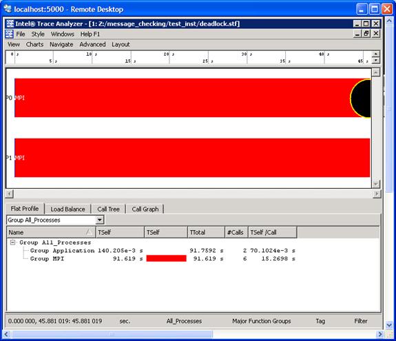
Figure 6.7 – Event Timeline illustrating an error as signified by the black circle
For the event timeline chart, errors and warnings are represented by yellow-bordered circles (Figure 6.7). The color of each circle depends on the type of the particular diagnostic. If there is an error the circle will be filled in with a black coloring. If there is a warning, the circle will be filled in with a gray coloring.
For Figure 6.7, error messages and warnings can be suppressed by using a context menu. A context menu will appear if you right click the mouse as shown in Figure 6.8 and follow the path Show->Issues. If you uncheck the Issues item, the black and gray circles will clear.
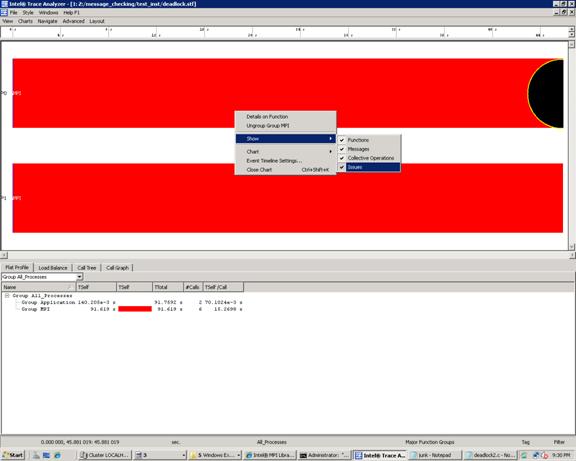
Figure 6.8 – Context menu that can be used to suppress “Issues”. This is done by un-checking the “Issues” item
One can determine what source line is associated with an error message by using the context menu and selecting Details on Function. This will generate the following Details on Function panel (Figure 6.9):
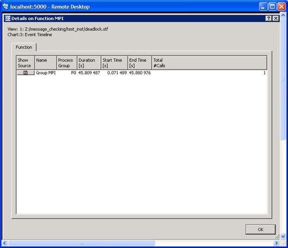
Figure 6.9 – Illustration of the Detail on Function panel. The Show Source tab is the first item on the left
If you click on the Show Source tab in Figure 6.9, you will ultimately reach a source file panel such as what is demonstrated in Figure 6.10.
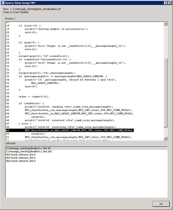
Figure 6.10 – The source panel display which shows the line in the user’s source where deadlock has taken place.
The diagnostic text messages and the illustration in Figure 6.10 reference line 49 of deadlock.c which looks something like the following:
…
49 MPI_Recv (buffer_in, MAX_ARRAY_LENGTH, MPI_INT, other, 999,
50 MPI_COMM_WORLD, &status);
51 MPI_Send (buffer_out, messagelength, MPI_INT, other, 999,
52 MPI_COMM_WORLD);
…
This is illustrated in Figure 6.11. To avoid deadlock situations, one might be able to resort to the following solutions:

1. Use a different ordering of MPI communication calls between processes
2. Use non-blocking calls
3. Use MPI_Sendrecv or MPI_Sendrecv_replace
4. Buffered mode
The If-structure for the original program looks something like the following:
…
41 if (sendfirst) {
42 printf ("\n%d/%d: sending %d\n", rank, size, messagelength);
43 MPI_Send (buffer_out, messagelength, MPI_INT, other, 999, MPI_COMM_WORLD);
44 MPI_Recv (buffer_in, MAX_ARRAY_LENGTH, MPI_INT, other, 999,
45 MPI_COMM_WORLD, &status);
46 printf ("\n%d/%d: received %d\n", rank, size, messagelength);
47 } else {
48 printf ("\n%d/%d: receiving %d\n", rank, size, messagelength);
49 MPI_Recv (buffer_in, MAX_ARRAY_LENGTH, MPI_INT, other, 999,
50 MPI_COMM_WORLD, &status);
51 MPI_Send (buffer_out, messagelength, MPI_INT, other, 999,
52 MPI_COMM_WORLD);
33 printf ("\n%d/%d: sendt %d\n", rank, size, messagelength);
54 }
…
If you replace lines 43 to 44 and lines 49 to 52 with calls to MPI_Sendrecv so that they look something like:
MPI_Sendrecv (buffer_out, messagelength, MPI_INT, other, 999, buffer_in, MAX_ARRAY_LENGTH, MPI_INT, other, 999, MPI_COMM_WORLD, &status);
and save this information into a file called deadlock2.c, and proceed to compile the modified application. The result of running the mpiexec command:
mpiexec -genv VT_CHECK_TRACING on -genv LD_PRELOAD libVTmc.so -genv VT_DEADLOCK_TIMEOUT 20s -genv VT_DEADLOCK_WARNING 25s -n 2 ./deadlock2.exe 0 80000
is the following:
…
0/2: receiving 80000
1/2: receiving 80000
0/2: sent 80000
1/2: sent 80000
[0] INFO: Error checking completed without finding any problems.
This indicates the deadlock errors that were originally encountered have been eliminated for this example. Using the Intel® Trace Analyzer to view the instrumentation results, we see that the deadlock issues have been resolved (Figure 6.12).
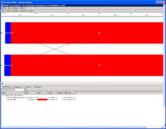
Figure 6.12 – Illustration of deadlock removal by using MPI_Sendrecv in the original source file called deadlock.c
6.6 Saving a Working Environment through a Project File
There may be situations where you are in the middle of an inspection with Intel® Trace Analyzer and you need to be away. For example, suppose you initially typed the command:
traceanalyzer test_inst/testcpp.stf
and you need to temporarily stop the analysis, and you are looking at the following panel:
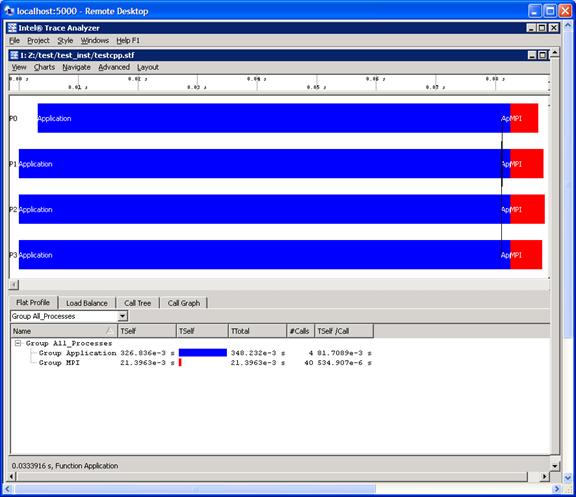
Figure 6.13 – Event timeline for running 4 MPI processes for the executable generated from test.cpp
For the panel rendering above, if you selection Project->Save Project or Project->Save Project As…, you will generate a subpanel that allows you to save the state of your session. This is project file has a suffix of “.itapr”, which is an acronym for Intel® Trace Analyzer project. Figure 6.14 shows the process of saving the state of your session through a project file.
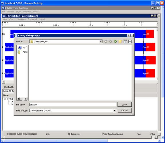
Figure 6.14 – Saving a Project File called testcpp.itapr
Suppose at a later time you wish to continue the analysis with Intel® Trace Analyzer. You can type the command:
traceanalyzer
You can then select Project->Load Project… and the following subpanel will appear (Figure 6.15):
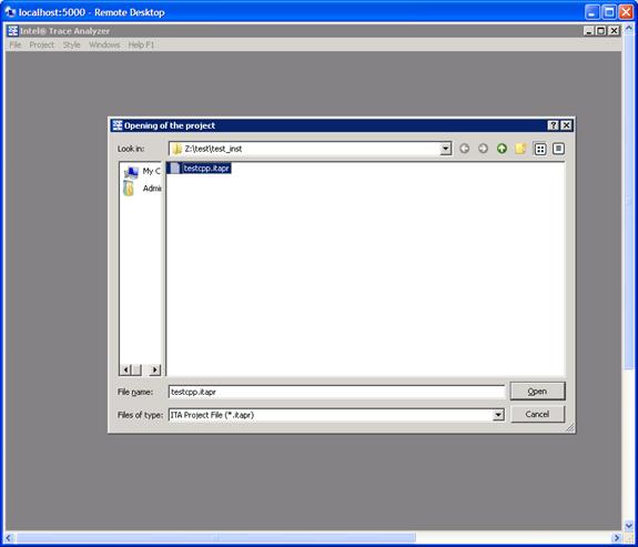
Figure 6.15 – Loading a Project File called testcpp.itapr
With regards to Figure 6.15, simply mouse over the Open button and you will immediately go back to point where you last left off (Figure 6.13). For complete details on saving and loading a project file, please see Section 2.2 of the Intel® Trace Analyzer Reference Guide, which is titled “Project Menu”. The path to this file is:
<directory-path-to-ITAC>/doc/ITA_Reference_Guide.pdf
on the system where the Intel® Trace Analyzer and Collector is installed.
6.7 Analysis of Application Imbalance
With respect to Figure 6.13, a developer may want to know a summary of process imbalance for the executable. One can do this by selecting the menu path Advanced->Application Imbalance Diagram. Figure 6.16 shows the result of making this selection.
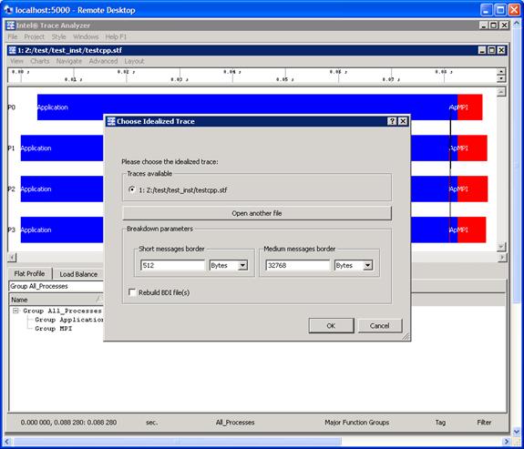
Figure 6.16 – Selecting Application Imbalance for the menu selection Advanced->Application Imbalance Diagram
Pressing the OK button in the subpanel will generate the following (Figure 6.17). You can verify the meaning of the histogram subcomponents by pressing on the Colors… button in Figure 6.17. This will generate the panel shown in Figure 6.18.
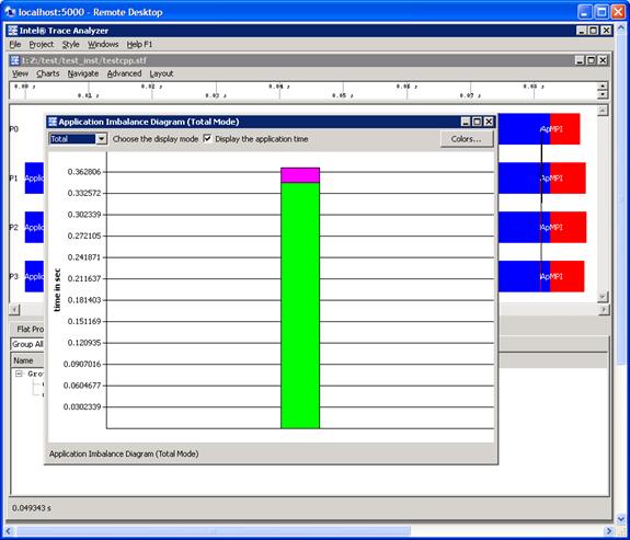
Figure 6.17 – Histogram subpanel as a result of pressing the OK button shown in Figure 6.16
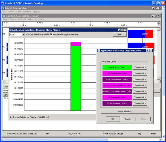
Figure 6.18 – Legend for interpreting the histogram contributions for the Application Imbalance Diagram
For complete details on application imbalance, please see Section 5.4 of the Intel® Trace Analyzer Reference Guide, which is titled “Application Imbalance Diagram Dialog Box”. The path to this file is:
<directory-path-to-ITAC>/doc/ITA_Reference_Guide.pdf
on the system where the Intel® Trace Analyzer and Collector is installed.
6.8 Analysis with the Ideal Interconnect Simulator
In analyzing the performance of your executable, you can compare your instrumentation trace with an ideal trace for the executable. To do this, make the menu selection Advanced->Idealized. As a result of this, a dialog subpanel will appear which will allow you to create an idealized trace of execution (Figure 6.19):
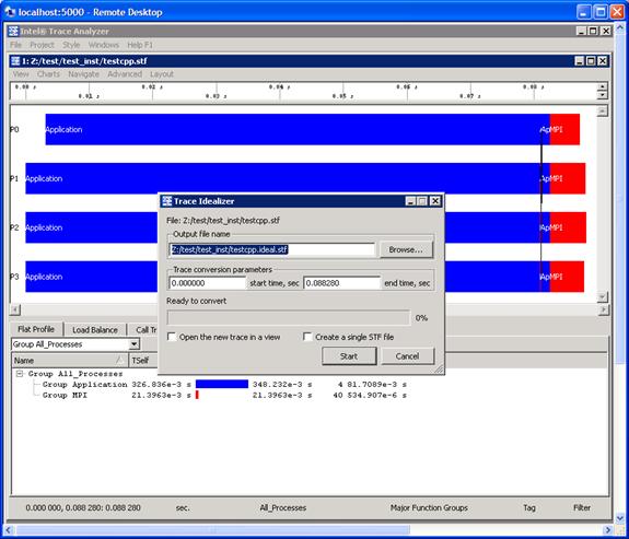
Figure 6.19 – Trace Idealizer dialog box generated as a result of the menu selection Advanced->Idealization
By pressing the Start button in the dialog panel for Figure 6.19, a trace file will be generated called “testcpp.ideal.stf”. After creating this file, you can then make the menu selection File->Open for the given Intel® Trace Analyzer panel and open the trace file “testcpp.ideal.stf” for comparative analysis. Figure 6.20 shows the side-by-side results of the actual execution trace and the ideal trace for the application “test.cpp”.
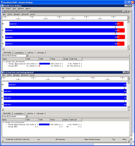
Figure 6.20 – Comparison of the actual execution trace versus the idealized trace for the application test.cpp
Notice in Figure 6.20 that the cost of doing message passing in the ideal case is negligible. You can use the data from the ideal case to help gauge the type of tuning performance that should be pursued.
For complete details on application imbalance, please see Section 5.3 of the Intel® Trace Analyzer Reference Guide, which is titled “Trace Idealizer Dialog Box”. The path to this file is:
<directory-path-to-ITAC>/doc/ITA_Reference_Guide.pdf
on the system where the Intel® Trace Analyzer and Collector is installed.
6.9 Building a Simulator with the Custom Plug-in Framework
Intel® Trace Analyzer and Collector provides you with a custom plug-in API that allows you to write your own simulator. The simulator API can be find in the folder path:
<directory-path-to-ITAC>/examples/icpf/
on the system where the Intel® Trace Analyzer and Collector is installed. The API source file within the subfolder icpf is called h_devsim.cpp. For background on building a customer simulator for trace files, please see Chapter 9 of the Intel® Trace Analyzer Reference Guide, which is titled “Custom Plug-in Framework”. The path to this file is:
<directory-path-to-ITAC>/doc/ITA_Reference_Guide.pdf
On Linux-based platforms, the installation process for Intel MKL on the cluster system will produce a sub-directory that looks something like .../mkl where the build number 017 may vary. The default directory path for the library installation process is:
/opt/intel/ictce/4.0.0.017/mkl
The contents of the .../mkl sub-directory should be:
benchmarks/
doc/
examples/
include/
interfaces/
lib/
licenses/
man/
tests/
tools/
uninstall.sh
Complete user documentation for Intel Math Kernel Library 10.2 can be found within the directory path:
<directory-path-to-mkl>/doc
where <directory-path-to-mkl> is the absolute directory path to where the Intel MKL files and sub-directories are installed on the cluster system.
To experiment with the ScaLAPACK test suite, recursively copy the contents of the directory path:
<directory-path-to-mkl>/tests/scalapack
to a scratch directory area which is sharable by all of the nodes of the cluster. In the scratch directory, issue the command:
cd scalapack
You can type the command:
gmake libem64t mpi=intelmpi30 LIBdir=<directory-path-to-mkl>/lib/em64t
Note that the gmake command above is applicable to Intel® 64 processor-based systems. This makefile creates and runs executables for the ScaLAPACK (SCAlable LAPACK) examples.
<directory-path-to-mkl>/tests/scalapack/source/TESTING
Finally, for IA-32 architectures, the gmake command might be:
gmake lib32 mpi=intelmpi30 LIBdir=<directory-path-to-mkl>/lib/32
In the scalapack working directory where the gmake command was issued, the ScaLAPACK executables can be found in source/TESTING, and the results of the computation will be placed into a sub-directory called _results. The _results directory will be created in same directory from which the gmake command was launched. Within this folder is another sub-folder which has a naming convention that uses the following makefile variable configuration:
_$(arch)_$(mpi)_$(comp)_$(opt)$(ADD_IFACE)
For example, on Intel® 64 architecture, using Intel MPI Library 4.0, the Intel Compiler and no compiler optimization, the sub-directory under _results might be called:
_em64t_intelmpi30_intel_noopt_lp64
The “*.txt” files for the execution results can be found here. You can invoke an editor to view the results in each of the “*.txt” files that have been created.
As an example result, the file “cdtlu_em64t_intelmpi30_intel_noopt_lp64.txt” might have something like the following in terms of contents for an execution run on a cluster using 4 MPI processes. The cluster that generated this sample output consisted of 4 nodes. The text file was generated by the corresponding executable xcdtlu_em64t_intelmpi30_intel_noopt_lp64.
![]()
|
SCALAPACK banded linear systems. 'MPI machine'
Tests of the parallel complex single precision band matrix solve The following scaled residual checks will be computed: Solve residual = ||Ax - b|| / (||x|| * ||A|| * eps * N) Factorization residual = ||A - LU|| / (||A|| * eps * N) The matrix A is randomly generated for each test.
An explanation of the input/output parameters follows: TIME : Indicates whether WALL or CPU time was used. N : The number of rows and columns in the matrix A. bwl, bwu : The number of diagonals in the matrix A. NB : The size of the column panels the matrix A is split into. [-1 for default] NRHS : The total number of RHS to solve for. NBRHS : The number of RHS to be put on a column of processes before going on to the next column of processes. P : The number of process rows. Q : The number of process columns. THRESH : If a residual value is less than THRESH, CHECK is flagged as PASSED Fact time: Time in seconds to factor the matrix Sol Time: Time in seconds to solve the system. MFLOPS : Rate of execution for factor and solve using sequential operation count. MFLOP2 : Rough estimate of speed using actual op count (accurate big P,N).
The following parameter values will be used: N : 3 5 17 bwl : 1 bwu : 1 NB : -1 NRHS : 4 NBRHS: 1 P : 1 1 1 1 Q : 1 2 3 4
Relative machine precision (eps) is taken to be 0.596046E-07 Routines pass computational tests if scaled residual is less than 3.0000
TIME TR N BWL BWU NB NRHS P Q L*U Time Slv Time MFLOPS MFLOP2 CHECK ---- -- ------ --- --- ---- ----- ---- ---- -------- -------- -------- -------- ------
WALL N 3 1 1 3 4 1 1 0.000 0.0001 1.06 1.00 PASSED WALL N 5 1 1 5 4 1 1 0.000 0.0001 1.75 1.66 PASSED WALL N 17 1 1 17 4 1 1 0.000 0.0001 6.10 5.77 PASSED WALL N 3 1 1 2 4 1 2 0.000 0.0003 0.36 0.53 PASSED WALL N 5 1 1 3 4 1 2 0.000 0.0002 0.90 1.35 PASSED WALL N 17 1 1 9 4 1 2 0.000 0.0002 3.03 4.59 PASSED WALL N 3 1 1 2 4 1 3 0.001 0.0006 0.19 0.27 PASSED WALL N 5 1 1 2 4 1 3 0.001 0.0010 0.17 0.30 PASSED WALL N 17 1 1 6 4 1 3 0.001 0.0010 0.75 1.16 PASSED WALL N 3 1 1 2 4 1 4 0.001 0.0007 0.17 0.24 PASSED WALL N 5 1 1 2 4 1 4 0.002 0.0026 0.08 0.13 PASSED WALL N 17 1 1 5 4 1 4 0.001 0.0011 0.66 1.00 PASSED
Finished 12 tests, with the following results: 12 tests completed and passed residual checks. 0 tests completed and failed residual checks. 0 tests skipped because of illegal input values.
END OF TESTS. |
![]()
The text in the table above reflects the organization of actual output that you will see.
Please recall from Intel MPI Library and Intel Trace Analyzer and Collector discussions that the above results are dependent on factors such as the processor type, the memory configuration, competing processes, and the type of interconnection network between the nodes of the cluster. Therefore, the results will vary from one cluster configuration to another.
If you proceed to load the cdtlu_em64t_intelmpi30_intel_noopt_lp64.txt table above into a Microsoft Excel* Spreadsheet, and build a chart to compare the Time in Seconds to Solve the System (SLV) and the Megaflop values, you might see something like the following (Figure 7.1):
Figure 7.1 – Display of ScaLAPACK DATA from the executable xcdtlu_em64t_intelmpi30_intel_noopt_lp64
7.1 Gathering Instrumentation Data and Analyzing the ScaLAPACK Examples with the Intel® Trace Analyzer and Collector
In the chapter entitled Interoperability of Intel MPI Library with the Intel® Trace Analyzer and Collector, cursory explanations were provided in gathering trace data and opening various analyzer panels for viewing trace-file content. Analysis of the ScaLAPACK examples with Intel Trace Collector and Intel Trace Analyzer can also be done easily. This subsection will dwell further on the instrumentation and analysis process. The discussion will focus on how to alter the command-line options for the ScaLAPACK gmake command so that performance data collection will be possible. Note however, that you will want to have plenty of disk storage available for collecting trace information on all of the examples because there are approximately 68 ScaLAPACK executables. To instrument the ScaLAPACK examples on an IA-32 cluster that is running Linux, you could use the following gmake command:
gmake lib32 mpi=intelmpi30 LIBdir=/opt/intel/ictce/4.0.0.017/mkl/lib/32 INSLIB="-L${VT_LIB_DIR} -lVT ${VT_ADD_LIBS}"
Finally, for the Intel® 64 architecture, the gmake command for gathering ScaLAPACK instrumentation data on Linux could possibly be:
gmake libem64t mpi=intelmpi30 LIBdir=/opt/intel/ictce/4.0.0.017/mkl/lib/em64t INSLIB="-L${VT_LIB_DIR} -lVT ${VT_ADD_LIBS}"
For all three command-line examples listed above, the make file variable INSLIB is used to specify the library path name and the libraries used for instrumentation by the Intel® Trace Collector. The variable name INSLIB is simply an acronym for instrumentation library.
Recall the instrumentation processes discussed in Chapter 6. The recommended amount of disk storage for collecting trace data on all of the ScaLAPACK test cases is about 5 gigabytes. For an executable such as xzevc_em64t_intelmpi30_intel_noopt_lp64 located in source/TESTING that has been instrumented with the Intel Trace Collector, a trace file called xzevc_em64t_intelmpi30_intel_noopt_lp64.stf will be generated. For the gmake commands above, the STF files will also be located in the sub-directory path source/TESTING and the summary reports for each ScaLAPACK executable will be placed under a sibling directory path to source called _results. Recalling the protocol that was discussed in the chapter for using Intel Trace Analyzer, you can proceed to analyze the content of xzevc_em64t_intelmpi30_intel_noopt_lp64.stf with the following shell command:
traceanalyzer xzevc_em64t_intelmpi30_intel_noopt_lp64.stf &
This command for invoking the Intel Trace Analyzer will cause the Event Timeline Chart and the Function Profile Chart (Figure 7.2) to be produced as described previously:
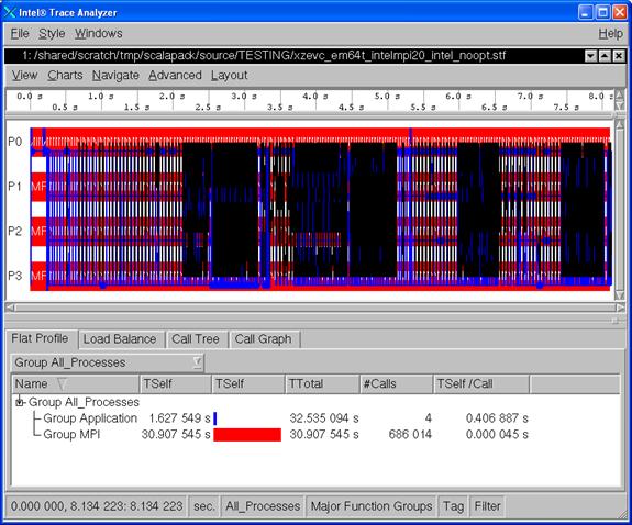
Figure 7.2 – Event Timeline Chart and the Function Profile Chart for the executable xzevc_em64t_intelmpi30_intel_noopt_lp64
By default, the ScaLAPACK makefile uses 4 MPI processes. If you wish to decrease or increase the number of MPI processes, you can adjust the MPIRUN makefile variable. An example for doing this on a system based on Intel® 64 architecture might be the following:
gmake libem64t mpi=intelmpi30 LIBdir=/opt/intel/ictce/4.0.0.017/mkl/lib/em64t MPILIB="-L${VT_LIB_DIR} -lVT ${VT_ADD_LIBS}" MPIRUN="mpiexec -n 6"
You should again realize that the contents of a trace file such as xzevc_em64t_intelmpi30_intel_noopt_lp64.stf will vary from cluster configuration to cluster configuration due to factors such as the processor type, the memory configuration, competing processes, and the type of interconnection network between the nodes of the cluster.
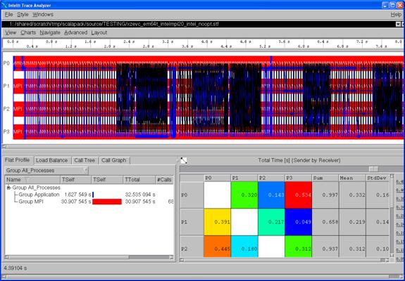
Figure 7.3 – The Message Profile Chart (lower right) for the executable xzevc_em64t_intelmpi30_intel_noopt_lp64
If you proceed to select Charts->Message Profile, you will generate the Message Profile Chart shown in Figure 7.3. Subsequently, if Charts->Collective Operations Profile is selected, then the chart shown in Figure 7.4 will be produced.
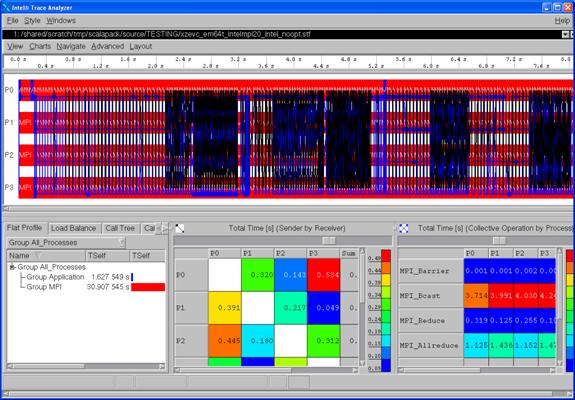
Figure 7.4 – Display of the Collective Operations Profile Chart (lower right) for xzevc_em64t_intelmpi30_intel_noopt_lp64
You can zoom in on a particular time interval for the Event Timeline Chart in Figure 7.4. Clicking on the left-most mouse button and panning across the desired time interval will cause the zoom in function. For example, Figure 7.5 shows zooming in to the time interval which spans from approximately 3.0 seconds to approximately 3.01 seconds. Notice that the number of message lines that are shown in black in Figure 7.5 is significantly reduced with respect to Figure 7.4.
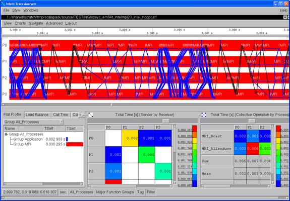
Figure 7.5 – Zooming in on the Event Timeline Chart for example xzevc_em64t_intelmpi30_intel_noopt_lp64
For Figure 7.5, the blue collective operation communication lines can be “drilled-down-to” by using the context menu as shown in Figure 7.6 in order to view the collective operation.
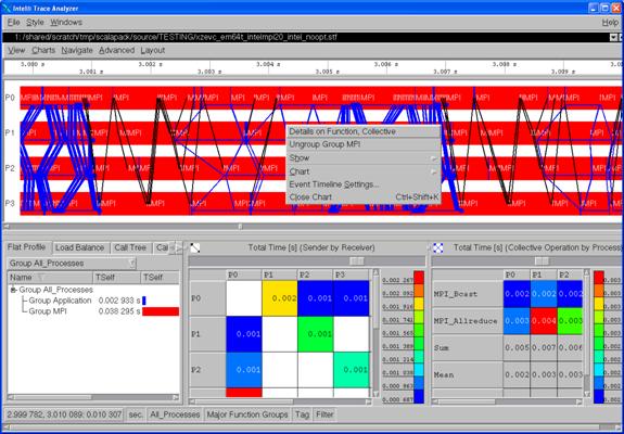
Figure 7.6 – Context Menu Selection for starting the process of drilling down to what the particular collective operation was executing (e.g. MPI_Allreduce) within the executable xzevc_em64t_intelmpi30_intel_noopt_lp64
If you would like to do a drill-down to actual source, the source files used to build the executables would have to be compiled with the –g option, and the Intel Trace Collector VT_PCTRACE environment variable would have to be set. For the ScaLAPACK gmake command, you might set the –g option with the following makefile variable:
OPTS="-O0 -g"
7.2 Experimenting with the Cluster DFT Software
On Linux OS, in the directory path:
<directory-path-to-mkl>/examples
you will find a set of sub-directories that look something like:
./ cdftc/ fftw2x_cdft/ interval/ pdepoissonf/ versionquery/
../ cdftf/ fftw2xf/ java/ pdettc/ vmlc/
blas/ dftc/ fftw3xc/ lapack/ pdettf/ vmlf/
blas95/ dftf/ fftw3xf/ lapack95/ solver/ vslc/
cblas/ fftw2xc/ gmp/ pdepoissonc/ spblas/ vslf/
The two sub-directories that will be discussed here are cdftc and cdftf. These two directories respectively contain C and Fortran programming language examples of the Cluster Discrete Fourier Transform (CDFT). To do experimentation with the contents of these two folders, a sequence of shell commands could be used to create instrumented executables and result information. For the C language version of the CDFT, the Bourne Shell or Korn Shell commands might look something like:
|
Intel Processor Architecture |
Command-line Sequence for Linux |
Trace Results are Located In |
Execution Results are Located In |
|
IA-32 |
#!/bin/sh export CWD=${PWD} export VT_LOGFILE_PREFIX=${CWD}/cdftc_inst rm -rf ${VT_LOGFILE_PREFIX} mkdir ${VT_LOGFILE_PREFIX} export VT_PCTRACE=5 export VT_DETAILED_STATES=5 cd /usr/local/opt/intel/ictce/4.0.0.017/mkl/examples/cdftc gmake lib32 mpi=intel3 workdir=${VT_LOGFILE_PREFIX} CS="mpiicc -t=log" RS="mpiexec -n 4" RES_DIR=${VT_LOGFILE_PREFIX} |
${CWD}/cdftc_inst |
${CWD}/cdftc_inst |
|
Intel® 64 (formerly Intel EM64T) |
#!/bin/sh export CWD=${PWD} export VT_LOGFILE_PREFIX=${CWD}/cdftc_inst rm -rf ${VT_LOGFILE_PREFIX} mkdir ${VT_LOGFILE_PREFIX} export VT_PCTRACE=5 export VT_DETAILED_STATES=5 cd /usr/local/opt/intel/ictce/4.0.0.017/mkl/examples/cdftc gmake libem64t mpi=intel3 workdir=${VT_LOGFILE_PREFIX} CS="mpiicc -t=log" RS="mpiexec -n 4" RES_DIR=${VT_LOGFILE_PREFIX} |
${CWD}/cdftc_inst |
${CWD}/cdftc_inst |
where <directory-path-to-mkl>/examples in the shell command-sequence above is:
/usr/local/opt/intel/ictce/4.0.0.017/mkl/examples
Note that the folder path above will vary depending on where the Intel Cluster Toolkit Compiler Edition was installed on your system. The change directory command above (i.e. cd …) transfers the Bourne Shell or Korn Shell session to:
/usr/local/opt/intel/ictce/4.0.0.017/mkl/examples/cdftc
The gmake command for the target lib32 is one contiguous line that ends with CS="mpiicc -t=log". This command references the makefile variables lib32, mpi, workdir, CS, and RS. As mentioned above, the target for the gmake command is lib32. The other target of this type is libem64t. The target libem64t is for Intel® 64 architecture. The makefile variable CS is set so that the resulting executable is linked against the logging versions of Intel MPI and the Intel Trace Collector. The RS makefile variable allows you to control the number of MPI processes. The default for RS is “mpiexec –n 2” when using Intel MPI Library. You can get complete information about this makefile by looking at its contents. There is also a help target built within the makefile, and therefore you can type:
gmake help
Assuming that ${CWD} has been defined from above for the Fortran language version of the CDFT, the Bourne Shell or Korn Shell commands might look something like:
|
Intel Processor Architecture |
Command-line Sequence for Linux |
Trace Results are Located In |
Execution Results are Located In |
|
IA-32 |
export VT_LOGFILE_PREFIX=${CWD}/cdftf_inst rm -rf ${VT_LOGFILE_PREFIX} mkdir ${VT_LOGFILE_PREFIX} export VT_PCTRACE=5 export VT_DETAILED_STATES=5 cd /usr/local/opt/intel/ict/4.0.0.017/mkl/examples/cdftf gmake lib32 mpi=intel3 workdir=${VT_LOGFILE_PREFIX} CS="mpiifort -t=log -DMPI_KIND_=4" RS="mpiexec -n 4" RES_DIR=${VT_LOGFILE_PREFIX}" |
${CWD}/cdftf_inst |
${CWD}/cdftf_inst |
|
Intel® 64 (formerly Intel EM64T) |
export VT_LOGFILE_PREFIX=${CWD}/cdftf_inst rm -rf ${VT_LOGFILE_PREFIX} mkdir ${VT_LOGFILE_PREFIX} export VT_PCTRACE=5 export VT_DETAILED_STATES=5 cd /usr/local/opt/intel/ict/4.0.0.017/mkl/examples/cdftf gmake libem64t mpi=intel3 workdir=${VT_LOGFILE_PREFIX} CS="mpiifort -t=log -DMPI_KIND_=4" RS="mpiexec -n 4" RES_DIR=${VT_LOGFILE_PREFIX} |
${CWD}/cdftf_inst |
${CWD}/cdftf_inst |
If you consolidate the shell script commands for performing C and Fortran Cluster Discrete Fourier computation on a particular Intel processor architecture, say Intel® 64 architecture, the complete Bourne shell script content might look something like:
#!/bin/sh
export CWD=${PWD}
export VT_LOGFILE_PREFIX=${CWD}/cdftc_inst
rm -rf ${VT_LOGFILE_PREFIX}
mkdir ${VT_LOGFILE_PREFIX}
export VT_PCTRACE=5
export VT_DETAILED_STATES=5
cd /usr/local/opt/intel/ict/4.0.0.017/mkl/examples/cdftc
gmake libem64t mpi=intel3 workdir=${VT_LOGFILE_PREFIX} CS="mpiicc -t=log" RS="mpiexec -n 4" RES_DIR=${VT_LOGFILE_PREFIX}
export VT_LOGFILE_PREFIX=${CWD}/cdftf_inst
rm -rf ${VT_LOGFILE_PREFIX}
mkdir ${VT_LOGFILE_PREFIX}
export VT_PCTRACE=5
export VT_DETAILED_STATES=5
cd /usr/local/opt/intel/ict/4.0.0.017/mkl/examples/cdftf
gmake libem64t mpi=intel3 workdir=${VT_LOGFILE_PREFIX} CS="mpiifort -t=log -DMPI_KIND_=4" RS="mpiexec -n 4" RES_DIR=${VT_LOGFILE_PREFIX}
After executing the shell script above, the ${CWD}/cdftc_inst and ${CWD}/cdftf_inst folders should contain the respective executables and the output results. The executable and result contents of each folder path might look something like:
dm_complex_2d_double_ex1.exe
dm_complex_2d_double_ex2.exe
dm_complex_2d_single_ex1.exe
dm_complex_2d_single_ex2.exe
and
dm_complex_2d_double_ex1.res
dm_complex_2d_double_ex2.res
dm_complex_2d_single_ex1.res
dm_complex_2d_single_ex2.res
The files with the suffix .res are the output results. A partial listing for results file called dm_complex_2d_double_ex1.res might be something like:
|
Program is running on 4 processes
DM_COMPLEX_2D_DOUBLE_EX1 Forward-Backward 2D complex transform for double precision data inplace
Configuration parameters:
DFTI_FORWARD_DOMAIN = DFTI_COMPLEX DFTI_PRECISION = DFTI_DOUBLE DFTI_DIMENSION = 2 DFTI_LENGTHS (MxN) = {20,12) DFTI_FORWARD_SCALE = 1.0 DFTI_BACKWARD_SCALE = 1.0/(m*n) …
Compute DftiComputeForwardDM
Forward result X, 4 columns
Row 0: ( 1.000, 0.000)( 1.000, 0.000)( 1.000, 0.000)( 1.000, 0.000) ( 1.000, 0.000)( 1.000, 0.000)( 1.000, 0.000)( 1.000, 0.000) ( 1.000, 0.000)( 1.000, 0.000)( 1.000, 0.000)( 1.000, 0.000) Row 1: ( 1.000, 0.000)( 1.000, 0.000)( 1.000, 0.000)( 1.000, 0.000) ( 1.000, 0.000)( 1.000, 0.000)( 1.000, 0.000)( 1.000, 0.000) ( 1.000, 0.000)( 1.000, 0.000)( 1.000, 0.000)( 1.000, 0.000) Row 2: ( 1.000, 0.000)( 1.000, 0.000)( 1.000, 0.000)( 1.000, 0.000) ( 1.000, 0.000)( 1.000, 0.000)( 1.000, 0.000)( 1.000, 0.000) ( 1.000, 0.000)( 1.000, 0.000)( 1.000, 0.000)( 1.000, 0.000) Row 3: ( 1.000, 0.000)( 1.000, 0.000)( 1.000, 0.000)( 1.000, 0.000) ( 1.000, 0.000)( 1.000, 0.000)( 1.000, 0.000)( 1.000, 0.000) ( 1.000, 0.000)( 1.000, 0.000)( 1.000, 0.000)( 1.000, 0.000) Row 4: ( 1.000, 0.000)( 1.000, 0.000)( 1.000, 0.000)( 1.000, 0.000) ( 1.000, 0.000)( 1.000, 0.000)( 1.000, 0.000)( 1.000, 0.000) ( 1.000, 0.000)( 1.000, 0.000)( 1.000, 0.000)( 1.000, 0.000) Row 5: ( 1.000, 0.000)( 1.000, 0.000)( 1.000, 0.000)( 1.000, 0.000) ( 1.000, 0.000)( 1.000, 0.000)( 1.000, 0.000)( 1.000, 0.000) ( 1.000, 0.000)( 1.000, 0.000)( 1.000, 0.000)( 1.000, 0.000) Row 6: ( 1.000, 0.000)( 1.000, 0.000)( 1.000, 0.000)( 1.000, 0.000) ( 1.000, 0.000)( 1.000, 0.000)( 1.000, 0.000)( 1.000, 0.000) ( 1.000, 0.000)( 1.000, 0.000)( 1.000, 0.000)( 1.000, 0.000) Row 7: ( 1.000, 0.000)( 1.000, 0.000)( 1.000, 0.000)( 1.000, 0.000) ( 1.000, 0.000)( 1.000, 0.000)( 1.000, 0.000)( 1.000, 0.000) ( 1.000, 0.000)( 1.000, 0.000)( 1.000, 0.000)( 1.000, 0.000) Row 8: ( 1.000, 0.000)( 1.000, 0.000)( 1.000, 0.000)( 1.000, 0.000) ( 1.000, 0.000)( 1.000, 0.000)( 1.000, 0.000)( 1.000, 0.000) ( 1.000, 0.000)( 1.000, 0.000)( 1.000, 0.000)( 1.000, 0.000)
…
|
Also, the setting of the environment variable VT_LOGFILE_PREFIX within the shell script results in the deposit of trace information into the directories cdftc_inst and cdftf_inst as demonstrated with a listing of the Structured Trace Format (STF) index files:
cdftc_inst/dm_complex_2d_double_ex1.exe.stf
cdftc_inst/dm_complex_2d_double_ex2.exe.stf
cdftc_inst/dm_complex_2d_single_ex1.exe.stf
cdftc_inst/dm_complex_2d_single_ex2.exe.stf
and
cdftf_inst/dm_complex_2d_double_ex1.exe.stf
cdftf_inst/dm_complex_2d_double_ex2.exe.stf
cdftf_inst/dm_complex_2d_single_ex1.exe.stf
cdftf_inst/dm_complex_2d_single_ex2.exe.stf
You can issue the following Intel Trace Analyzer shell command to initiate performance analysis on cdftc_inst/dm_complex_2d_double_ex1.exe.stf:
traceanalyzer ./cdftc_inst/dm_complex_2d_double_ex1.exe.stf &
Figure 7.7 shows the result of simultaneously displaying the Function Profile Chart and the Event Timeline Chart.
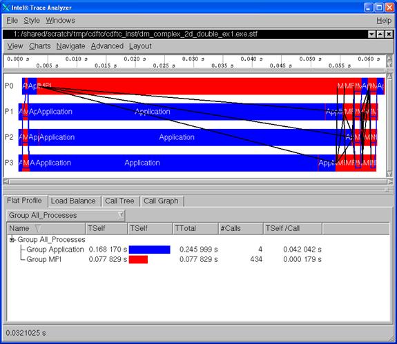
Figure 7.7 – The Event Timeline Chart and the Function Profile Chart for a Cluster Discrete Fourier Transform Example
7.3 Experimenting with the High Performance Linpack Benchmark
On Linux, in the directory path:
<directory-path-to-mkl>/benchmarks/mp_linpack
you will find a set of files and subdirectories that look something like the following:
./ COPYRIGHT* INSTALL* Make.ia32* man/ src/ www/
../ HISTORY* lib_hybrid/ Make.ipf* nodeperf.c* testing/
bin_intel/ HPL.build.log.220120040613* Make.em64t* makes/ README* TODO*
BUGS* include/ Makefile* Make.top* setup/ TUNING*
If you make a scratch directory, say:
test_mp_linpack
on a file share for your cluster, and copy the contents of <directory-path-to-mkl>/benchmarks/mp_linpack into that scratch directory you can then proceed to build a High Performance Linpack executable. To create an executable for Intel® 64 architecture, you might issue the following gmake command:
gmake arch=em64t LAdir=/usr/local/opt/intel/ictce/4.0.0.010/mkl/lib/em64t LAinc=/usr/local/opt/intel/ictce/4.0.0.010/mkl/include
where the command sequence above is one continuous line. The macros LAdir and LAinc describe the directory path to the Intel® 64 Math Kernel library and the Intel® MKL include directory, respectively. The partial directory path /usr/local/opt/intel/ictce/4.0.0.010 for the macros LAdir and LAinc should be considered an example of where an Intel® Math Kernel Library might reside. Note that on your system, the path and a version number value such as 4.0.0.010 may vary depending on your software release.
The High Performance Linpack executable for the gmake command above will be placed into …/test_mp_linpack/bin/em64t and will be called xhpl. The table below summarizes makefile and associated mpiexec commands that might be used to create xhpl executables for IA-32, and Intel® 64 architectures, respectively. The command-line syntax in the table is that of Bourne* Shell or Korn* Shell. The mpiexec commands use 4 MPI processes to do the domain decomposition.
|
Intel Processor Architecture |
Command-line Sequence for Linux |
Executable is Located In |
Execution Results are Located In |
|
IA-32 |
#!/bin/sh export CWD=${PWD} gmake clean_arch_all arch=ia32 gmake arch=ia32 LAdir=/usr/local/opt/intel/ictce/4.0.0.010/mkl/lib/32 LAinc=/usr/local/opt/intel/ictce/4.0.0.010/mkl/include cd ${CWD}/bin/ia32 mpiexec –n 4 ./xhpl > results.ia32.out 2>&1 |
${CWD}/bin/ia32 |
${CWD}/bin/ia32 |
|
Intel® 64 (formerly Intel EM64T) |
#!/bin/sh export CWD=${PWD} gmake clean_arch_all arch=em64t gmake arch=em64t LAdir=/usr/local/opt/intel/ictce/4.0.0.010/mkl/lib/em64t LAinc=/usr/local/opt/intel/ictce/4.0.0.010/mkl/include cd ${CWD}/bin/em64t mpiexec –n 4 ./xhpl > results.em64t.out 2>&1 |
${CWD}/bin/em64t |
${CWD}/bin/em64t |
The output results might look something like the following for Intel® 64 architecture:
|
================================================================================ HPLinpack 2.0 -- High-Performance Linpack benchmark -- September 10, 2008 Written by A. Petitet and R. Clint Whaley, Innovative Computing Laboratory, UTK Modified by Piotr Luszczek, Innovative Computing Laboratory, UTK Modified by Julien Langou, University of Colorado Denver ================================================================================
An explanation of the input/output parameters follows: T/V : Wall time / encoded variant. N : The order of the coefficient matrix A. NB : The partitioning blocking factor. P : The number of process rows. Q : The number of process columns. Time : Time in seconds to solve the linear system. Gflops : Rate of execution for solving the linear system.
The following parameter values will be used:
N : 1000 NB : 112 120 PMAP : Row-major process mapping P : 1 2 1 4 Q : 1 2 4 1 PFACT : Left NBMIN : 4 2 NDIV : 2 RFACT : Crout BCAST : 1ring DEPTH : 0 SWAP : Mix (threshold = 256) L1 : no-transposed form U : no-transposed form EQUIL : no ALIGN : 8 double precision words
-------------------------------------------------------------------------------- …
================================================================================ T/V N NB P Q Time Gflops -------------------------------------------------------------------------------- WR00C2L2 1000 120 4 1 0.35 1.894e+00 -------------------------------------------------------------------------------- ||Ax-b||_oo/(eps*(||A||_oo*||x||_oo+||b||_oo)*N)= 0.0052671 ...... PASSED ============================================================================
Finished 16 tests with the following results: 16 tests completed and passed residual checks, 0 tests completed and failed residual checks, 0 tests skipped because of illegal input values. ----------------------------------------------------------------------------
End of Tests. ============================================================================
|
The file <directory-path-to-mkl>/doc/mkl_documentation.htm contains a landing page linking various documentation files associated with Intel MKL 10.2. To make inquiries about Intel Math Kernel Library 10.2, visit the URL: http://premier.intel.com.
8. Using the Intel® MPI Benchmarks
The Intel MPI Benchmarks have been ported to Linux*. The directory structure for the Intel® MPI Benchmarks 3.2 looks something like the following where the parenthesized text contains descriptive information:
- ./doc (ReadMe_IMB.txt; IMB_Users_Guide.pdf, the methodology description)
- ./src (program source code and Makefiles)
- ./license (Source license agreement, trademark and use license agreement)
- ./versions_news (version history and news)
- ./WINDOWS (Microsoft* Visual Studio* projects)
The WINDOWS folder as noted above contains Microsoft* Visual Studio* 2005 and 2008 project folders which allow you to use a pre-existing ".vcproj" project file in conjunction with Microsoft* Visual Studio* to build and run the associated Intel® MPI Benchmark application. Note that this is not relevant to Linux*.
If you type the command gmake within the src subdirectory, then you will get general help information that looks something like the following:
IMB_3.2 does not have a default Makefile any more.
This Makefile can be used to
gmake clean
For installing, please use:
gmake -f make_ict
to install the Intel(r) Cluster Tools (ict) version.
When an Intel(r) MPI Library install and mpiicc path exists,
this should work immediately.
Alternatively, use
gmake -f make_mpich
to install an mpich or similar version; for this,
you normally have to edit at least the MPI_HOME
variable provided in make_mpich
To clean up the directory structure, in the directory src, simply type:
gmake clean
To compile the Intel MPI Benchmarks with the Intel Cluster Tools, simply type the command:
gmake –f make_ict
The three executables that will be created with the all target are:
IMB-EXT
IMB-IO
IMB-MPI1
Assuming that you have a four node cluster, and the Bourne Shell is being used simply type the commands:
mpiexec -n 4 IMB-EXT > IMB-EXT.report 2>&1
mpiexec -n 4 IMB-IO > IMB-IO.report 2>&1
mpiexec -n 4 IMB-MPI1 > IMB-MPI1.report 2>&1
Similarly, if C Shell is the command-line interface, type the commands:
mpiexec -n 4 IMB-EXT >&! IMB-EXT.report
mpiexec -n 4 IMB-IO >&! IMB-IO.report
mpiexec -n 4 IMB-MPI1 >&! IMB-MPI1.report
The Intel® C++ and Intel® Fortran Compilers on Linux have the command-line switch called -tcollect which allows functions and procedures to be instrumented during compilation with Intel® Trace Collector calls. This compiler command-line switch accepts an optional argument to specify the Intel® Trace Collector library to link with.
|
Library Selection |
Meaning |
How to Request |
|
libVT.a |
Default library |
-tcollect |
|
libVTcs.a |
Client-server trace collection library |
-tcollect=VTcs |
|
libVTfs.a |
Fail-safe trace collection library |
-tcollect=Vtfs |
Recall once again that in the test_intel_mpi folder for Intel MPI Library, there are four source files called:
test.c test.cpp test.f test.f90
To build executables with the -tcollect compiler option for the Intel Compilers, one might use the following compilation and link commands:
mpiicc test.c -tcollect -g -o testc_tcollect
mpiicpc test.cpp -g -tcollect -o testcpp_tcollect
mpiifort test.f -tcollect -g -o testf_tcollect
mpiifort test.f90 -tcollect -g -o testf90_tcollect
The names of the MPI executables for the above command-lines should be:
testc_tcollect
testcpp_tcollect
testf_tcollect
testf90_tcollect
So as to make a comparison with the Intel Trace Collector STF files:
testc.stf testcpp.stf testf.stf testf90.stf
within the directory test_inst, we will use the following mpiexec commands:
mpiexec -n 4 -env VT_LOGFILE_PREFIX test_inst testc_tcollect
mpiexec -n 4 -env VT_LOGFILE_PREFIX test_inst testcpp_tcollect
mpiexec -n 4 -env VT_LOGFILE_PREFIX test_inst testf_tcollect
mpiexec -n 4 -env VT_LOGFILE_PREFIX test_inst testf90_tcollect
The corresponding STF data will be placed into the folder test_inst. To do a comparison between the STF data in testcpp.stf and testcpp_tcollect.stf the following traceanalyzer command can be launched from a Linux command-line panel within the folder test_intel_mpi:
traceanalyzer
Figure 13.1 shows the base panel for the Intel Trace Analyzer as a result of invoking the command above from a Linux panel.
Figure 9.1 – Base panel for the Intel Trace Analyzer when invoking a Linux Shell Command: traceanalyzer without any arguments
If you select the menu path File->Open and click on the test_inst folder, the following panel will appear:
Figure 9.2 – Open a Tracefile Rendering for the test_inst Folder where testcpp.stf has been Highlighted
Selecting testcpp.stf will generate a Flat Profile panel within the Intel Trace Analyzer session that might look something like the following.
Figure 9.3 – Flat Panel Display for test_inst\testcpp.stf
For the Flat Panel Display, if you select File->Compare the following sub-panel will appear.
Figure 9.4 – Sub-panel Display for Adding a Comparison STF File
Click on the “Open another file” button and select testcpp_tcollect.stf and then proceed to push on the Open button with your mouse.
Figure 9.5 – Sub-panel Activating the Second STF File for Comparison
Click on the Ok button in Figure 9.5 and the comparison display in Figure 9.6 will appear. In Figure 9.6, notice that the timeline display for testcpp_tcollect.stf (i.e. the second timeline) is longer than that of the top timeline display (testcpp.stf).
Figure 9.6 – Comparison of testcpp.stf and testcpp_tcollect.stf
At the bottom and towards the right of this panel there are two labels with the same name, namely, Major Function Groups. Click on the top label with this name, and a sub-panel will appear with the following information:
Figure 9.7 – “Function Group Editor for file A” Display (i.e, for file testcpp.stf)
Highlight the “All Functions” tree entry and press the Apply but in the low right corner of this panel. Then press the OK button. Repeat this process for the second Major Function Groups label at the bottom of the main Trace Analyzer panel. You should now see a panel rendering that looks something like:
Figure 9.8 – Comparison of STF Files testcpp.stf and testcpp_tcollect.stf after making the All Functions Selection
At the top of the display panel, if you make the menu selection Charts->Function Profile you will be able to see a function profile comparison (lower middle and lower right) for the two executables:
Figure 9.9 – Function Profile Sub-panels in the Lower Middle and Lower Right Sections of the Display for testcpp.stf and testcpp_tcollect.stf
Notice that the lower right panel (testcpp_tcollect.stf) has much more function profiling information than the lower middle panel (testcpp.stf). This is the result of using the -tcollect switch during the compilation process. You can proceed to do similar analysis with:
1) testc.stf and testc_tcollect.stf
2) testf.stf and testf_tcollect.stf
3) testf90.stf and testf90_tcollect.stf
Cluster OpenMP is only available on Linux platforms. The Intel® architecture must be Intel® 64. The application must be written with the C and/or Fortran programming languages.
The major advantage of Cluster OpenMP is that it facilitates ordinary OpenMP*-like parallel programming but on a distributed memory system where it uses the same fork/join, and shared memory model of parallelism that ordinary OpenMP uses. This methodology may be easier to use than message-passing paradigms such as MPI or PVM*.
OpenMP is a directive-based language that annotates an underlying serial program with parallel programming semantics. The underlying serial program runs sequentially when you turn off OpenMP directive processing within the Intel Compiler. With proper planning, you can develop your parallel application just as you would develop a serial program and then enable parallelism with OpenMP. Since you can parallelize your application in an increment fashion, OpenMP usually helps you write a parallel program more quickly and easily than you could with other techniques.
Unfortunately, not all programs are suitable for Cluster OpenMP. If your application meets the following two criteria, it may be a good candidate for using Cluster OpenMP parallelization:
1. Your application shows excellent speedup with ordinary OpenMP.
If the scalability of your application is poor with ordinary OpenMP on a single node, then porting it to Cluster OpenMP is not recommended. The scalability for Cluster OpenMP is in most cases worse than for ordinary OpenMP because Cluster OpenMP has higher overheads for almost all constructs, and sharable memory accesses can be costly. Ensure that your application gets good speedup with “ordinary” OpenMP before taking steps to use Cluster OpenMP.
To test for this condition, run the OpenMP form of the program (a program compiled with the -openmp Intel compiler option) on one node, once with one thread and once with n threads, where n is the number of processors on the single node.
For the most time-consuming parallel regions, if the speedup achieved for n threads is not close to n, then the code is not suitable for Cluster OpenMP. In other words, the following formula should be true:
Speedup = Time(1 thread) / Time(n threads) = ~n
Note that the formula above measures a scalability form of speedup. This measurement is not the same as the speedup that is associated with the quality of parallelization for a given application. That type of speedup is calculated as follows:
Speedup = Time(serial) / Time(n threads)
2. Your application has good locality of reference and little synchronization.
An OpenMP program that gets excellent speedup may get good speedup with Cluster OpenMP as well. However, the data access pattern of your application can make use of the Cluster OpenMP model scale poorly even if it scales well with ordinary OpenMP. For example, if a thread typically accesses large amounts of data that were last written by a different thread, or if there is excessive synchronization, a Cluster OpenMP program may spend large amounts of time sending messages between nodes, which can prevent good speedup.
If you are not sure whether your code meets these criteria, you can use the Cluster OpenMP utility called clomp_forecaster.pl that is described in Chapter 9.3 of the Cluster OpenMP Users Guide to see if Cluster OpenMP is appropriate for your application. The Cluster OpenMP Users Guide is located in:
.../cluster_omp/docs
with respect to the Intel C++ or Intel Fortran Compiler directory paths. Similarly, the utility clomp_forecaster.pl is located in:
.../cluster_omp/tools
10.1 Running Cluster OpenMP Examples
In the directory path for the Intel C++ Compiler:
.../samples
there is a subfolder called cluster. The content of that sub-directory is the following:
kmp_cluster.ini Makefile md.c README.txt
If you copy the contents of this directory to a shared area that is accessible by all of the nodes of the cluster, and provide an mpd.hosts file that is unique to your cluster, you can type:
gmake clean
gmake build
gmake run
Notice in regards to the makefile target build within the file Makefile for the command gmake build, that the Intel compiler switch –cluster-openmp is being used for the compilation of the C source file md.c. The gmake run command executes the following:
time md.exe > md.out
The output data is placed into the file md.out. The timing information might look something like:
real 0m31.563s
user 0m13.198s
sys 0m0.956s
Please note that the timing results that you achieve will at a minimum be a function of the number of nodes in the cluster, the interconnection fabric, the memory size, and the processor architecture.
Similarly for the directory path to the Intel Fortran Compiler:
.../samples/cluster
This sub-directory path contains:
kmp_cluster.ini Makefile md.f README.txt
Again, if you copy the contents of this directory to a shared area that is accessible by all of the nodes of the cluster, and provide an mpd.hosts file that is unique to your cluster, you can type:
gmake clean
gmake build
gmake run
When you issue the gmake build command for the Fortran version of the Cluster OpenMP example, you should see something like the following:
ifort -cluster-openmp md.f -o md.exe
As with the C programming example for Cluster OpenMP, the -cluster-openmp command-line switch instructs the Fortran compiler to use the Cluster OpenMP libraries. Similarly, regarding the gmake run command, the following target semantics will be invoked:
time md.exe > md.out
for the Fortran-based executable md.exe.
10.2 Gathering Performance Instrumentation Data and Doing Analysis with Intel® Trace Analyzer and Collector
The Intel Trace Analyzer and Collector can be used to help you analyze the performance of a Cluster OpenMP* application.
To use Intel Trace Analyzer and Collector with a Cluster OpenMP application use the following sequence of steps:
1. Ensure that your LD_LIBRARY_PATH includes the directory where the appropriate Intel Trace Analyzer dynamic libraries exist, normally in the directory path <directory-path-to-ITAC>/slib. Note that this is automatically solved if you source ictvars.csh or ictvars.sh when respectively using C Shell or Bourne Shell as your command-line interface.
2. Set the environment variable KMP_TRACE to the value 1.
3. Add the option “--IO=files” to the kmp_cluster.ini file.
4. Run your executable on a set of nodes.
Regarding the examples md.c and md.f in the last subsection, you can set following sequence of Bourne Shell commands assuming that you are using a Bourne Shell environment:
export KMP_TRACE=1
export VT_LOGFILE_PREFIX=${PWD}/inst
rm -rf ${VT_LOGFILE_PREFIX}
mkdir ${VT_LOGFILE_PREFIX}
time ./md.exe > md.out 2>&1
Recall that the environment variable VT_LOGFILE_PREFIX will direct instrumentation data into a directory path such as ${PWD}/inst. After execution of md.exe, the contents of ${PWD}/inst might look something like:
./ md.exe.prot md.exe.stf.dcl md.exe.stf.gop md.exe.stf.msg md.exe.stf.pr.0 md.exe.stf.sts
../ md.exe.stf md.exe.stf.frm md.exe.stf.gop.anc md.exe.stf.msg.anc md.exe.stf.pr.0.anc
As your application executes, it will produce trace file data which records important events that took place inside the Cluster OpenMP runtime library. You can analyze this trace file with Intel Trace Analyzer to tune and improve the performance of your application.
As with an MPI application, you can view the Cluster OpenMP performance data by running traceanalyzer with the trace filename as an argument. For example, the executable referenced above was called md.exe. Based on the contents of ${PWD}/inst for our example, the command-line for the trace analyzer from the directory ${PWD} might be:
traceanalyzer md.exe.stf
This will produce the profile display illustrated in Figure 10.1.
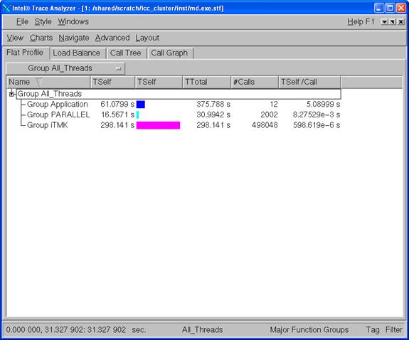
Figure 10.1 – Profile Display for trace file md.ex.stf
Figure 14.2 shows the result of opening up the Event Timeline display through the menu selection Charts->Event Timeline:
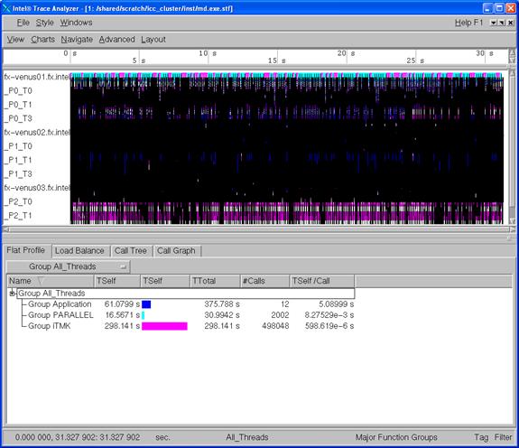
Figure 10.2 – Intel® Trace Analyzer display showing the Event Timeline and Function profile display for md.exe
Notice that there is a large concentration of black lines shown in Figure 10.2. This represents communication between the various processor threads. You can zoom in on a particular segment of the time line by using your mouse (leftmost button) and highlighting a particular time line interval (Figure 10.3).
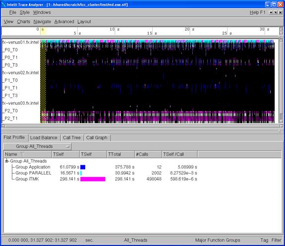
Figure 10.3 – Highlighting a time interval (shown in yellow) with the leftmost mouse button
Again, note that the results that you will see on your system will be at a minimum be a function of the number of nodes in the cluster, the interconnection fabric, the memory size, and the processor architecture.
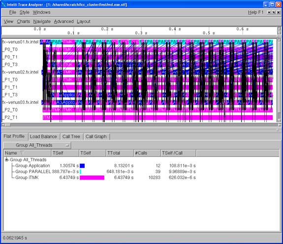
Figure 10.4 – The result of zooming on the particular time line segment that was highlighted in Figure 14.3
To make inquiries about Cluster OpenMP, visit the URL: http://whatif.intel.com. At the bottom of this landing page, there is a web link titled WhatIf Alpha Software Forums where you can review past questions, read what other people are working on, post a new inquiry, get support from product authors, and read the opinions of fellow users.