We have developed an interactive data language (IDL) reduction pipeline: Solvepol, to analyse polarimetric data acquired with the polarimeter POLIAG mounted on the 0.6-m telescope at Observatório do Pico dos Dias (OPD) operated by the Laboratório Nacional de Astrofísica (LNA) in Brazil. The pipeline will be free distribution (after extensive test) to be downloaded in the link bellow.

Pipeline: pipelineV16.1.tar.gz

About the drawer IAGPOL

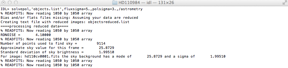
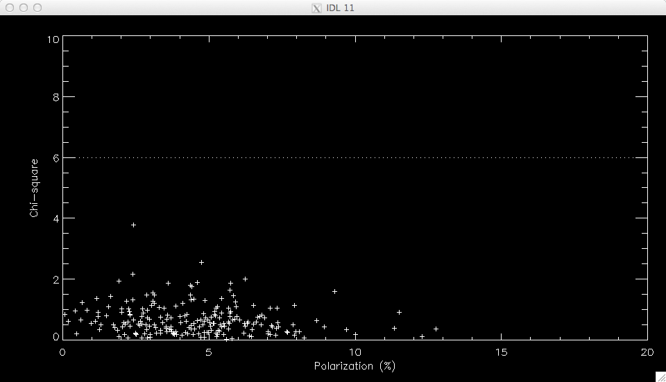
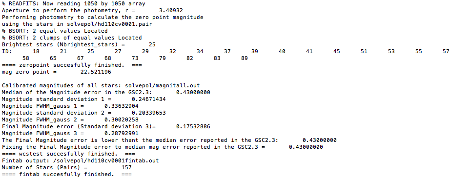
An example of the use of the Solvepol (pipelineV16.1) is presented. Please read the Manual for more information. This example consists in the reduction of the field centred on the standard star HD110984. The images of HD110984 are included in the tar.gz file. It is recommended that you run this pilot example to make sure that the pipeline is running correctly in your computer.

Example:

To run the pipeline type solvepol followed by the name of the file containing the list of images to analyse. The list have to be in order of the position angle of the waveplate (L0, L1, L2... etc, and not L3, L0, L2...). The name of the file listing the objects is "objects.list" (see figure bellow).

By default Solvepol uses a flux/sigma_flux ratio of 2.0 to find the sources. If you want a different value, set the optional input parameter fluxsigma to your value. In this example we chose fluxsigma = 5.

The default of the ratio polarisation/sigma_polarisation is 1.0. You can choose another value for the default setting the optional parameter polsigma. In this example we chose polsigma= 3.

Solvepol uses the Astronomy.net software to solve the astrometry. If your computer has Astrometry.net installed, you might want to run it in your local computer. To do so set the optional parameter astrometry = y or /astrometry. If the astrometry keyword is not set, the pipeline will prompt you to give the solution that you can get from the Astrometry.net web page (see the Manual for details). In the example we set /astrometry because we do have the Astrometry.net software installed in our computer.

Other keywords composing the pipeline will be explained at its time bellow. For the reduction keywords: nreads, bias and flats, see the Manual. They are not used in this example - the images are already reduced.

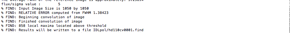
Solvepol calculates the average fwhm of thestars in the first position angle of the waveplate. The fwhm is used to find the sources using the IDL procedure find.pro.

If you know the fwhm in advance or you the fwhm calculated by Solvepol is not what you expect, you could set the optional keyword fwhm to your value. In the example the pipeline calculates a fwhm = 3.26 pixels (see image below), an expected value. But you whant to change the value for any reason, let's say, to fwhm = 5, the syntax to run Solvepol is:

IDL> solvepol,'objects.list',fluxsigma=5.,polsigma=3.,fwhm=5,/astrometry

We chose fluxsigma = 5. to find sources 5 times over the standard deviation of the sky.

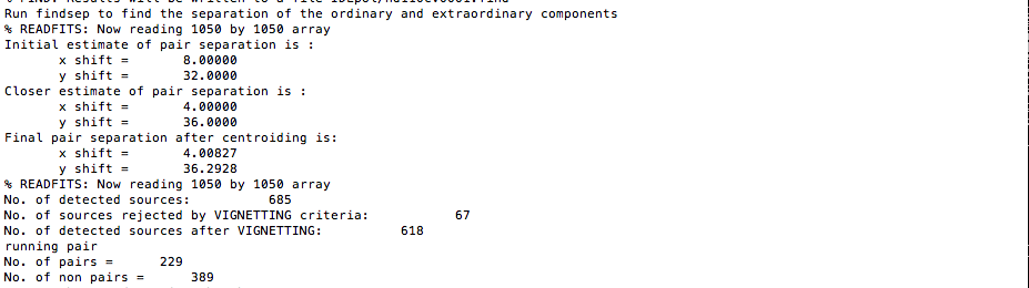
The pipeline will calculates the offsets in X and Y between the ordinary and extraordinary beams. However there are cases where these shifsts are not correctly calculated (we expect to be the least), and the correct values have to be provided. If the calculated shifs are 0.0 for both the offset in X and Y (clearly a wrong shift if the observations were properly executed with the Savart calcite), the pipeline will stop and you will be asked to give the correct values. Measure the offsets in X and Y between the ordinary and extraoridnary stars and provide the correct values. Press enter to continue. If the calculated shifts are not zero or some strange high values, the pipeline will continue without stopping.

The shift between images at the different position angles of the waveplate is calculated.

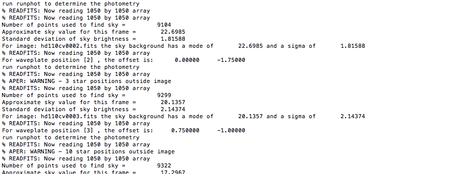
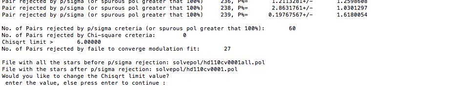
The photometry is performed within 10 concetric apertures at each waveplate position angle. We chose polsigma = 3, then surces with lower pol/sigma_pol values will be rejected. Also sources whose modulation cannot be fitted are rejected too.

The status and number of sources are printed along the running. The Chisqrt of the best fit to the modulation vs polarisation is ploted. All sources with Chisqrt greater than 6.0 are rejected. The pipeline will prompt you to change this value if you set the flag chisqrtint (chi-square interactively. Chose the chisqrt limit interactively by setting chisqrtint='y' or /chisqrtint). We found that 6.0 is a good limit to excude espurious polarisation after several tests on diferent fields. Therefore, 6.0 is the default limit of the Chi-square.

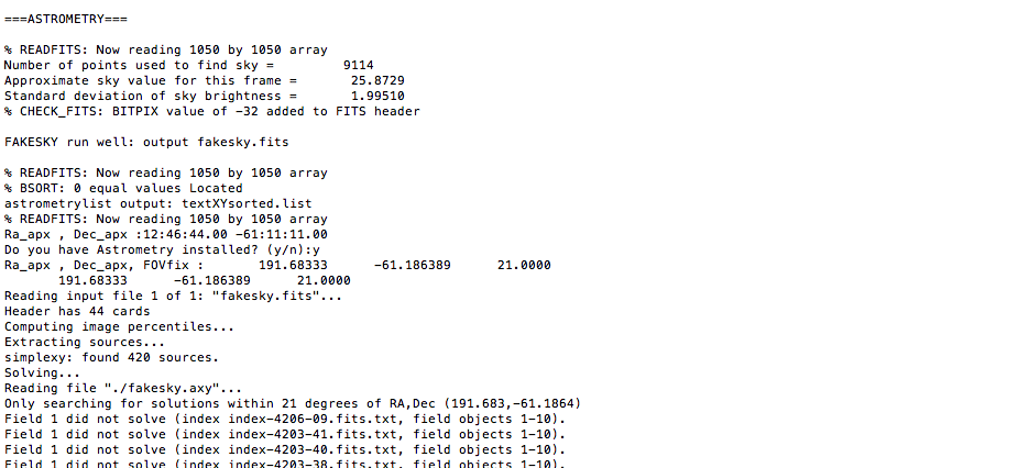
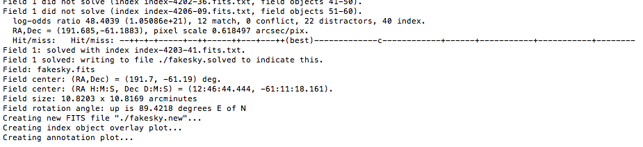
Astrometry.net is called to estimate the wcs. The pipeline asks whether you have Astrometry.net installed or not by setting the optional keyword astrometry. In our example we have indicated that we do have the Astrometry software installed.

The pipeline creates an image called fakesky.fits that has the ordinary stars masked out to facilitate the calculation of the astrometry and to being consitent with the chosen ordinary and estraordinary stars, and a list of the detected stars sorted out by brightness. If you do not have Astrometry.net, then enter the created textXYsorted.list file or the fakesky.fits into the Astrometry.net site manually, and give the output file of Astrometry.net that contains the astrometry solution in the header to the pipeline (fakesky.new.fits or wcs.fits).

The zero point magnitude is calibarted using the GSC2.3 catalogue via Vizier. Up to 25 stars are used to do the calibration. If there are no stars to calibrate, the zero point is set to zero (no magnitude calibration). The optical magnitudes and its error are estimated.

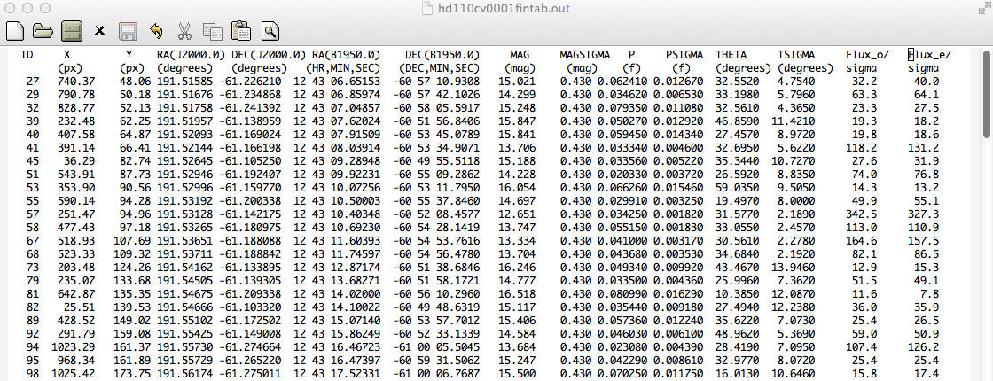
At this stage the final catalogue <name>fintab.out has been created.

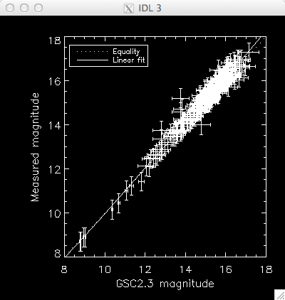
The calibrated magnitudes and the magnitudes from the GSC2.3 catalogue are plotted. A linear fit and the equality are oveploted.

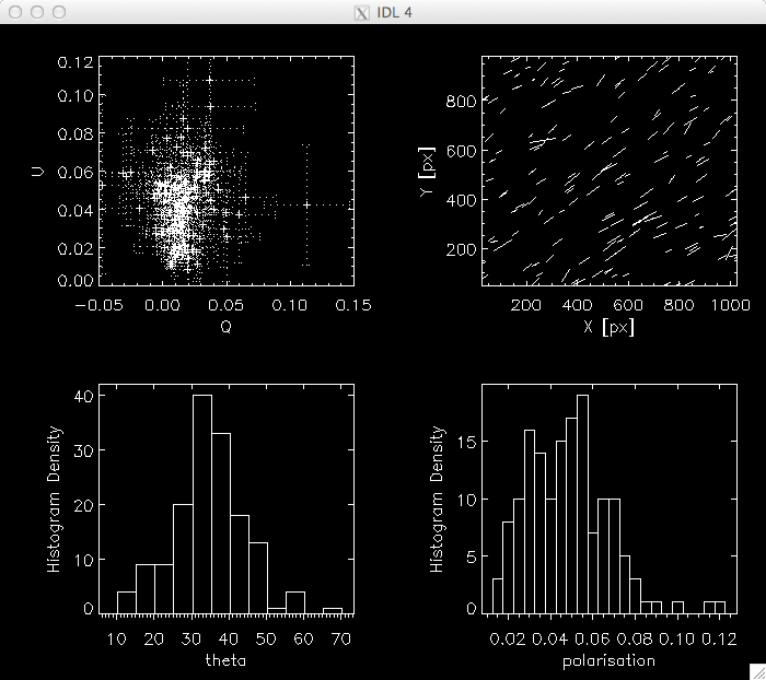
The Q-U space, a pixel map with the polarisation vectors and the desity distributions of theta and polarisation are plotted.

Other plots are generated: the density distribution of the magnitude, the polarisation vs magnitude and the error of the polarisation vs magnitude.

Solvepol gives you the option to overplot the IDs of the stars over the polarisation map for easier identification. We chose not to plot the IDs. To plot the IDs the syntax is:

IDL> solvepol,'objects.list',fluxsigma=5,polsigma=3,/astrometry,/oplotid

or

IDL> solvepol,'objects.list',fluxsigma=5,polsigma=3,/astrometry,oplotid=y

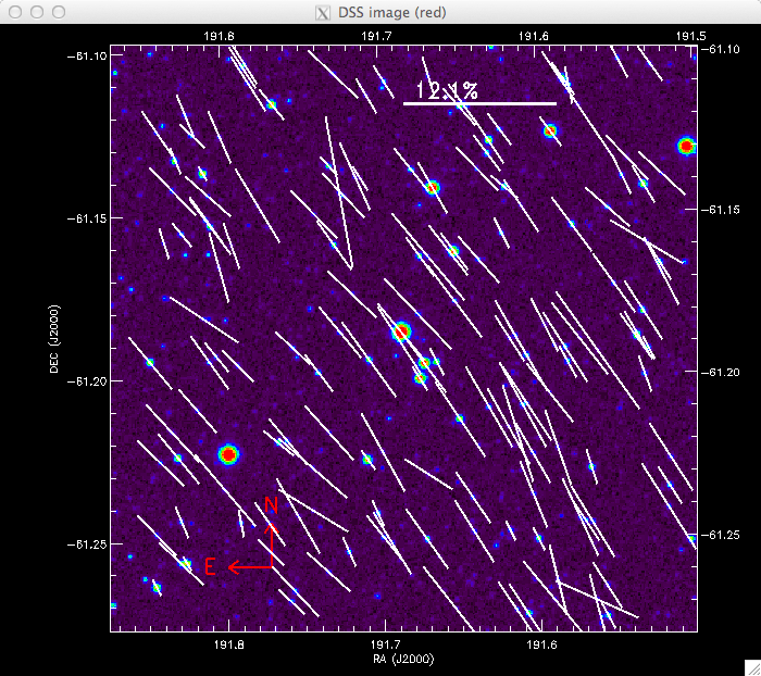
The polarisation map is plotted over the DSS R-band image.

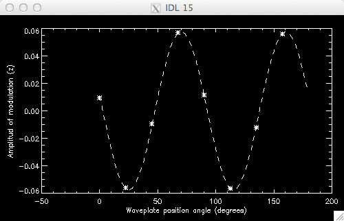
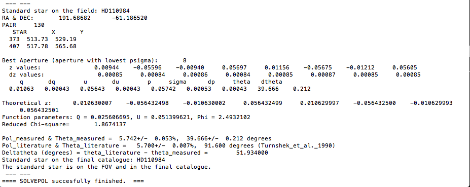
If your field contains a standard polarimetric star, it would be detected. The position angle correction Deltatheta is estimated and the modulation function vs the position angles of the waveplate is plotted. A log file solvepol.log is created (among other files and plots explained in Manual README.pdf).