First we'll get RAMSES and MUSIC:
git clone https://bitbucket.org/rteyssie/ramses/
hg clone https://bitbucket.org/ohahn/music
Then we'll compile RAMSES. First, enter the following folder:
cd ramses/binIn this folder you'll find the Makefile for the code. We'll need to edit two things in this Makefile. First, change
NDIM = 1to
NDIM = 3This tells RAMSES that we'll be running 3D simulations (it can also run 2D and 1D simulations). Then, comment the following lines like this:
# --- No MPI, gfortran -------------------------------
#F90 = gfortran -O3 -frecord-marker=4 -fbacktrace -ffree-line-length-none -g
#FFLAGS = -x f95-cpp-input $(DEFINES) -DWITHOUTMPI
and then uncomment the following ones like this, so that we end up with a parallelized version of RAMSES:
# --- MPI, gfortran syntax ------------------------------
F90 = mpif90 -frecord-marker=4 -O3 -ffree-line-length-none -g -fbacktrace
FFLAGS = -x f95-cpp-input $(DEFINES)
Then run make and you'll end up with an executable file called ramses3d.
Now let's compile MUSIC. Enter the folder
cd musicopen the Makefile and change the line that says HAVEHDF5 = yes to HAVEHDF5 = no. RAMSES doesn't support the HDF5 file format, so we don't need that. Then just compile with make and an executable named MUSIC will be created.
./MUSIC ics_example.confThis will generate a folder called ics_ramses containing the initial conditions. For more information about the configuration parameters, check out the user's guide.
&POISSON_PARAMS
epsilon=1.0d-4
/

&OUTPUT_PARAMS
delta_aout=0.01
aend=1.0
foutput=100
/

&CLUMPFIND_PARAMS
relevance_threshold=3
density_threshold=80.
saddle_threshold=-1.0
mass_threshold=10.
ivar_clump=0
clinfo=.true.
/
The last block isn't really necessary, but it's useful if you want to find the halos in your simulation (it will output text files with the locations of halos in the simulation at each snapshot). Also add the following line to the &RUN_PARAMS block in order to activate the clump finder:
clumpfind=.true.Now we're all set to start the simulation. Just run
mpirun -n 4 ./ramses3d ramses.nmlReplace the number of processors with the number of cores you have available/want to use (I'm assuming you're running on a quad-core computer).
$ pip install yt --user
The following script shows how you can use yt to load the positions and velocities of the particles in the simulation. It also outputs a csv file which can be read into datashader (see here what it does, you can also find there an example that works out of the box).
import yt
import numpy as np
import matplotlib.pyplot as plt

# loading the snapshot
ds = yt.load('output_00062/info_00062.txt')
ad = ds.all_data()

# reading particle positions and velocities into numpy arrays
pos = ad['particle_position']
vel = ad['particle_velocity']

# visualizing particle positions (ugly way)
plt.scatter(pos[:,0], pos[:,1], s=0.001)
plt.savefig('simple_visualization.png')

# writing particle positions to a csv file, which can be read
# into datashader
f = open('pos.csv', 'w')
f.write('x_col,y_col,z_col\n')
for i in pos:
  f.write('%f,%f,%f\n' % (i[0], i[1], i[2]))
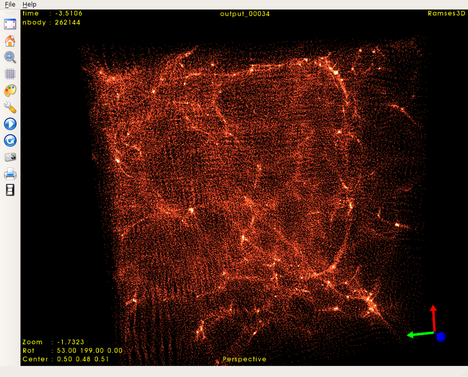
If you want to iteractively visualize the data, check out glnemo2: